Welcome to this weeks session on social network analysis!

Code

library(needs)
needs(igraph,
      intergraph,
      igraphdata)

Why study social groups?

An actor’s membership in highly cohesive social groups has been considered in many sociological studies. It has been hypothesised to correlate with other aspects of social behaviour such as

(Egoistic) suicide (Durkheim)
Adherence to social norms
Generalized trust
Access to human capital
Social status, authority, roles, and positions
Flow of information and influence

In order to empirically test these sorts of hypotheses, groups must be detected in a network.

But what exactly is a highly cohesive social group?

In network analysis, a social group can be defined by the structure of the underlying network relations. This task of identifying these is called community detection. The development of methods for community detection has been — and continues to be — a highly active area of research Smith and Papachristos (2021).

We look for groups (or communities) in networks because individuals often cluster together due to homophily (tendency to associate with similar others) or shared social contexts and activities. These structural clusters often play a critical role in shaping behavior, diffusion of information, and social influence.

By a community ,” we typically mean a set of nodes with dense internal connections and relatively few ties to the rest of the network (Kolaczyk and Csárdi 2020). This contrasts with overly strict definitions like cliques and better reflects the loosely cohesive groupings common in empirical networks .

Take for examples this artificially constructed network:

Code

# Create 3 groups with 10 nodes each
group_sizes <- c(20, 10, 10, 10)
num_groups <- length(group_sizes)

# Probability of connection
p_in <- 0.4  # high within-group connection probability
p_out <- 0.02  # low between-group connection probability


pref_matrix <- matrix(p_out,
                      nrow = num_groups,
                      ncol = num_groups)
diag(pref_matrix) <- p_in  # within-group connections

# Generate the graph using stochastic block model
g <- sample_sbm(sum(group_sizes),
                pref.matrix = pref_matrix,
                block.sizes = group_sizes)

# Add group membership as vertex attribute
V(g)$group <- rep(1:num_groups,
                  times = group_sizes)

# Color nodes by group
group_colors <- c("lavender", "lavender", "lavender", "lavender")
V(g)$color <- group_colors[V(g)$group]

# Plot the graph
plot(g,
     vertex.label = NA,
     vertex.size = 10,
     layout = layout_with_fr)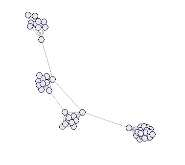

The detection is less trivial in most real networks.

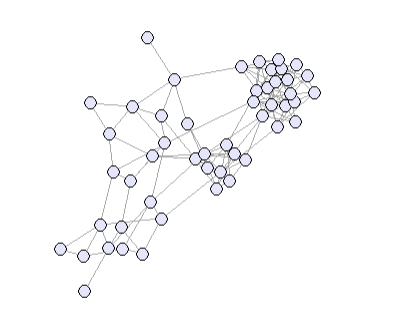
** Small world phenomenon**

In large scale contemporary societies, two randomly chosen individuals are personally connected, via their friends, acquaintances and family

A small-world network is thus a network that is characterized by

High clustering: your friends are also friends with each other.
Short average path lengths: most individuals are only a few steps away from one another.

Basic subgroup concepts

Subgroups in networks are often defined by patterns of connectivity. These patterns help us identify tightly knit sets of actors that may share similar roles, resources, or behaviors.

Cliques

One way to define network communities is by the level of connectivity. Recall that a network is completely connected if every pair of nodes is linked by a single edge.

Code

triad <- make_full_graph(3)  # Complete graph of 3 nodes (triad)
graph_4 <- make_full_graph(4)  # Complete graph of 4 nodes
graph_5 <- make_full_graph(5)  # Complete graph of 5 nodes
graph_6 <- make_full_graph(6)  # Complete graph of 6 nodes

par(mfrow = c(1, 4))

# Plot each graph
plot(triad, 
     vertex.size = 20, 
     vertex.label = NA, 
     vertex.color = "lavender", 
     edge.color = "gray")

plot(graph_4, 
     vertex.size = 20, 
     vertex.label = NA, 
     vertex.color = "lavender", 
     edge.color = "gray")

plot(graph_5, 
     vertex.size = 20, 
     vertex.label = NA, 
     vertex.color = "lavender", 
     edge.color = "gray")

plot(graph_6, 
     vertex.size = 20, 
     vertex.label = NA, 
     vertex.color = "lavender", 
     edge.color = "gray")

par(mfrow = c(1, 1))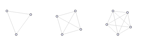

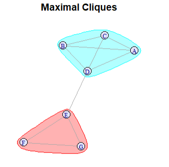
When applied to a subnetwork, such a structure is called a clique. A clique is maximal if no other actor can be added to it without breaking its complete connectivity. That is, every member is connected to every other, and no additional node outside the group is connected to all of them.

If you recall the triad-census from two weeks ago, a 3-clique is a triad 300 (Fuhse 2018).

For example, in the following network:

Code

g <- graph_from_literal(A:B:C:D -- A:B:C:D, D - E, E - F - G - E)

plot(g,
     layout = layout_with_fr,
     vertex.label.cex = 0.8,
     vertex.color = "lavender")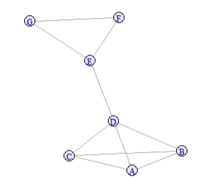

We can identify cliques and maximal cliques using:

Code

cliques(g,
        min = 3)

max_cliques(g,
            min = 3)

count_max_cliques(g,
                  min = 3)


largest_cliques(g)

# Visualize maximal cliques
plot(g,
     mark.groups = max_cliques(g, min=3),
     vertex.label.cex = 0.8,
     main = "Maximal Cliques",
     vertex.color="lavender")

# Visualize cliques
plot(g,
     mark.groups = cliques(g, min=3),
     vertex.label.cex = 0.8,
     main = "Cliques",
     vertex.color="lavender")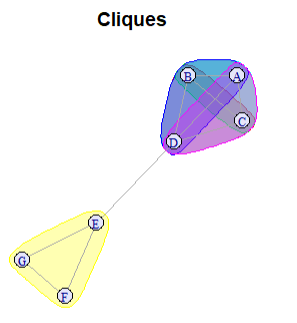

Create the following network:

Code

g <- graph_from_literal(1-2:3:4:5:6:7, 2-3:4:5:6:7, 3-4:5:6:7, 4-5:6:7,
                   5-6:7, 6-7, 7-8:9:10, 8-9:11,
                   11-12, 12-13:14, 9-10:13, 10-15,
                   14-16, 13-16, 15-16)

plot(g)

Identify all maximal cliques with min = 3 and highlight them visually

Assign the node IDs of the largest maximal clique to a variable called group.

Limitations of Cliques:

Cliques are one of the simplest and strictest forms of cohesive subgroups. However, they have several limitations:

The definition is conservative: cliques with more than three members are rare in real networks.
No internal differentiation: all members are structurally equivalent.
Computationally intractable for large networks.

n-Cliques

Cliques are oftenly connected with each other and nodes and relations overlap. Because of this, there are several proposals for the relaxation of these concepts (Balasundaram, Butenko, and Hicks 2011). One method is the so called n-clique. To identify these, we do not only count direct relationships, but we look at cliques as the clique and all nodes that are reachable within a distance of \(n\). Usually we call for small \(n\)s like \(2\).

Exercise:

Identify all nodes that are part of the 2-clique of the largest maximal clique of \(g\) and add them to the groupvariable

Code

dist_matrix <- distances(g, v = largest_clique)

dist <- apply(dist_matrix,
              2,
              min)

nodes <- which(dist <= 2)

V(g)$group[nodes] <- TRUE


V(g)$color <- ifelse(V(g)$group, "lavender", "lightblue")

plot(g)

k-Core Subgraphs

Another possibility to identify looser subgraphs are k-cores.

A k-core subgraph is a maximal subnetwork in which every node is connected to at least \(k\) other nodes within that subnetwork (Batagelj and Zaversnik 2003). The k-core of a graph is the maximal subgraph in which every vertex has at least degree k. The cores of a graph form layers: the (k+1)-core is always a subgraph of the k-core.

In igraph coreness() calculates the largest \(k\) (Coreness) for each node, so that this node belongs to this k-core.

Code

coreness(g)

K-Plex subgraphs

The concept of k-plex looks for the largest group \(n\) inside a network where each person is allowed to not know up to \(k-1\) persons in the group. So, each person must have at least \(n-k\) friends within the group.

Example: In a 2-plex of 5 people, everyone must know at least three of the others.

I graph doesn’t have a built-in support for k-plexes.

We can write our own function using the concepts of cliques though.

Code

all_cliques <- cliques(g, min = 4)


is_kplex <- function(graph, nodes, k) {
  subg <- induced_subgraph(graph, nodes)
  degs <- degree(subg)
  n <- length(nodes)
  all(degs >= (n - k))
}


k <- 2
kplexes <- Filter(function(nodes) is_kplex(g, nodes, k), all_cliques)

plot(g,
     mark.groups = kplexes,
     vertex.label.cex = 0.8,
     main = "2-Plex",
     vertex.color="lavender")

Cohesive groups

Another widely used approach to dividing a network into communities is based on the idea that members of a social group are more strongly connected to each other than to the rest of the network.

One way to formalize this is through structural cohesion. According to Moody and White (2003), the cohesion of a subnetwork can be defined by the extent to which its connectedness depends on individual members. That is, the structural cohesion of a group is measured by the minimum number of nodes that must be removed to disconnect the group.

This concept corresponds to vertex-connectivity (denoted as \(k\)): A group’s cohesion is the minimum number of actors who, if removed, would disconnect the group.

Moody and White proposed using this concept to divide a network into cohesive blocks — nested groups of actors that remain connected even as nodes are progressively removed.

“For a given graph g, a subset of its vertices h is said to be maximally k-cohesive if there is no superset of h with vertex connectivity greater than or equal to k”. Cohesive blocks are the maximally k-cohesive subnetworks.

In igraph we can find cohesive blocks via the call cohesive_blocks(). Through the graphs_from_cohesive_blocksgraphs_from_cohesive_blocks-function we can save these blocks as graphs. cohesion will give us the \(k\) score of each block. And max_cohesion()the maximal cohesion of each vertex.

However, the calculation of cohesive blocks is only efficient for small graphs (n < 100)

Code

b <- cohesive_blocks(g)
length(b) # number of cohesive blocks
blocks(b) # blocks as vectors
graphs_from_cohesive_blocks(b, g) # blocks as graphs

cohesion(b) # the cohesion of the blocks
max_cohesion(b) # the maximal cohesion of each vertex

Exercise:

“If your method doesn’t work on this network, then go home.”

– Eric Kolaczyk, at the opening workshop of the 2010-11 SAMSI program year on Complex Networks on the karate network

Zachary (1977) studied conflict and fission in this network, as the karate club was split into two separate clubs, after long disputes between two factions of the club, one led by John A., the other by Mr. Hi. The Faction vertex attribute gives the faction memberships of the actors. After the split of the club, club members chose their new clubs based on their factions, except actor no. 9, who was in John A.’s faction but chose Mr. Hi’s club.

Because the Karate-network from Zachary includes a real-life slpit, it gives a ground thruth to compare the algoritmic results.

Load the karate network from the igraphdata package

Code

data(karate)

plot(karate)

karate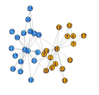

Karate-network: The color represents the faction

Use the described methods to identify subgroups in the graph.

Code

largest_clique <- largest_cliques(karate)
sapply(largest_cliques, length)

V(karate)$group_clique <- V(karate) %in% largest_clique

table(
  Clique = V(g)$group_clique,
  Truth = V(g)$truth
)

2.1 How well do they perform in reference to the ground truth?

2.2 What insight does each method provide?

Community detection algorithms

Although the general principle behind community detection is relatively straightforward - to identify those vertices that are more closely tied to each other than to others in the network - finding communities can be computationally very demanding - especially for large networks. Nevertheless, many algorithms have been developed and igraph contains several of them. With your own data you should try using different ones to determine which appears to be the most useful as they all have different strengths and weaknesses. In this section, you will use two different methods - the fast-greedy method and the edge-betweeness method.

Communities via edge betweenness

One intuitive way to identify communities is to find and remove the “bridges” between groups. These are the edges that lie on many shortest paths — in other words, they have high edge betweenness.

Edge betweenness is defined similarly to vertex betweenness:

Let
- \(( g_{jk} )\) be the number of shortest paths between nodes \(( j )\) and \(( k )\),
- \(( g_{jk}(e) )\) the number of those paths that pass through edge \(( e )\).

Then the edge betweenness \(( B(e) )\) is:

\[ B(e) = \sum_{j < k} \frac{g_{jk}(e)}{g_{jk}} \]

This metric helps identify key connectors in a network whose removal will fragment the graph.

Code

edge_betweenness(karate)

E(g)$betw <- edge_betweenness(karate)

plot(g,
     vertex.color = "lavender",  
     edge.label = E(karate)$betw ,  
     edge.color = "gray",  
     main = "Network with Edge Betweenness",
     vertex.size = 10,  # Set a reasonable node size
     vertex.label = NA,  # Hide node labels (optional),
     layout = layout_nicely(karate)
)

The Girvan-Newman Method

This algorithm uses edge betweenness to divide the network:

Calculate edge betweenness for all edges.
Remove the edge with the highest betweenness (Random selection if multiple candidates).
Recalculate betweenness.
Repeat until the network is split into components.

Although intuitive and sociologically grounded, this method is computationally expensive for large networks.

Code

eb <- cluster_edge_betweenness(karate)

# Number of communities found
length(eb)

# Community structure
communities(eb)
membership(eb)

# Visualize communities
plot(karate, mark.groups = communities(eb), main = "Girvan–Newman Communities")

Modularity based

Modularity is a quality measure for a particular division of a network into communities. It quantifies how well the division captures dense internal connections and sparse external ones. In other words the modularity score is an index of how inter-connected edges are within versus between communities.

Values of modularity range from −0.5 to 1, with higher values indicating clearer group structure. Values above ~0.3 usually indicate meaningful structure.

Modularity can also be used descriptively — for example, to assess how well a node attribute (e.g., gender, location) explains community divisions.

Fast and Greedy Algorithm

Fast-greedy is a modularity based method - it works by trying to build larger and larger communities by adding vertices to each community one by one and assessing a modularity score at each step.

It starts with each node as its own community
Then it looks for the best merge (If they are connected they will make the network more tightly connected)
Once the best pair of communities is found it merges them into a single community
Repeat until the algorithm can no longer find beneficial merges. (When all groups are as tightly knit as possible.)

Greedy: The algorithm is greedy because it always tries to make the best local decision at each step — merging the communities that will immediately improve the network’s structure.

Fast: It’s fast because it doesn’t have to check every possible community; it only considers the best possible merges, making the process quick.

In igraph, a relatively fast greedy algorithm is implemented that searches over all possible partitions and optimises the modularity in form of an agglomerative hierarchical clustering (Clauset, Newman, and Moore 2004)

Code

fgc <-cluster_fast_greedy(karate)

modularity(fgc)
membership(fgc)

plot(fgc, karate, main = "Fast Greedy Communities")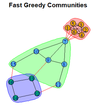

Louvain

(Nutarelli 2024)

The Louvain method is widely used for large networks.

It starts by trying to maximize the \(Q^t\) value (modularity). It reaches its peak when three conditions are met:

The delta term is one, indicating that \(i\) and \(j\) belong to the same communiry.
The \(\text{Adj}_{ij}\) is also 1 - suggesting a direct connection between two nodes
The fraction with ks (relates to the degree of nodes) is as small as possible. (Represents the expected number of edges between i and j if they were randomly connected).

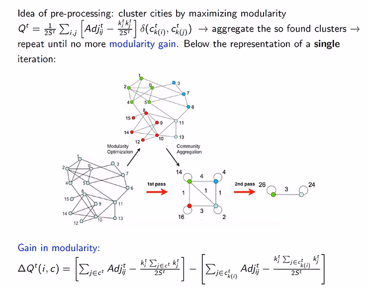
The louvain clustering algorithm

Maximizes the modularity: So it looks at all the connections between pairs of nodes and figures out how to group them into clusters in a way that maximizes the overall modularity
Forming supernodes: Once we have our initial clusters, we treat each cluster as if it where a single large node. This simplifies the network.
Iterative refinement: The process is then repeated. We look at this simpler network and again try to find the best way to group these big nodes into clusters. With each iteration, we’re looking to increase the modularity, refining the network’s structure.

We keep doing this until we can’t improve the modularity any further – in other words, until our clusters are as meaningful and well-defined as they can be.

This iterative process of clustering, creating big nodes, and then re-clustering allows the Louvain algorithm to efficiently and effectively reveal the underlying structure of complex networks.

Code

lv <- cluster_louvain(g)

modularity(lv)
plot(lv, g, main = "Louvain Communities")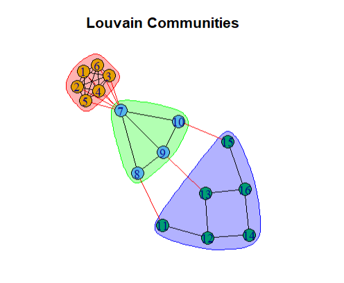

Pros:

Fast and scalable
Tends to detect modular structure well

Cons:

May yield slightly inconsistent results (depends on tie-breaking order)

Leiden

The Leiden algorithm improves Louvain by fixing some of its flaws (e.g., disconnected subcommunities). It guarantees well-connected communities and higher modularity while being fixer and more consistent as the Louvain.

The Leiden algorithm starts from a singleton partition
The algorithm moves individual nodes from one community to another to find a partition, c) which is then refined+.
An aggregate network is created based on the refined partition, using the non-refined partition to create an initial partition for the aggregate network.For example, the red community in (b) is refined into two subcommunities in (c), which after aggregation become two separate nodes in (d), both belonging to the same community.
The algorithm then moves individual nodes in the aggregate network
In this case, refinement does not change the partition .

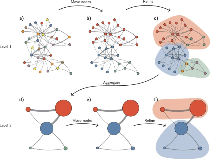
These steps are repeated until no further improvements can be made.

Code

lc <- cluster_leiden(g,
                     objective_function = "modularity",
                     n_iterations = 10)

#modularity
communities(lc)
membership(lc)

plot(lc, g, main = "Leiden Communities")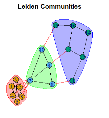

Further community detection algorithms implemented in `igraph`

Name	Function	Directed Ties	Weights	More Components
Edge-betweenness	`cluster_edge_betweenness`	✅	✅	✅
Leading eigenvector	`cluster_leading_eigen`	❌	❌	✅
Fast-greedy	`cluster_fast_greedy`	❌	✅	✅
Louvain	`cluster_louvain`	❌	✅	✅
Walktrap	`cluster_walktrap`	❌	✅	❌
Label propagation	`cluster_label_prop`	❌	✅	❌
InfoMAP	`cluster_infomap`	✅	✅	✅
Spinglass	`cluster_spinglass`	❌	✅	❌
Optimal	`cluster_optimal`	❌	✅	✅

Getting community information

Each community detection function produces several pieces of information in a community object. Using the functions length(), sizes() and membership() it is possible to quickly extract information about how many communities there are and which vertices are in which community. In igraph, it is also possible to make quick plots of the network which show each vertex in its community by color. To do this, the community object and graph object are included as the two arguments to the plot function.

Validation of Community

The problem of validating a network partitioning is not trivial. If a vertex attribute is suspected to correlate with the clustering, it can be used to validate the clustring.

Exercise:

Find communities in the karate network with the Girvan Newman method, the Louvain Algorithm and the Leiden algorithm.

Code

lc <- cluster_leiden(karate,
                     objective_function = "modularity",
                     n_iterations = 10)
plot(lc, karate)


cl <- cluster_leiden(karate,
                     objective_function = "modularity",
                     n_iterations = 10)
plot(cl, karate)



cfg <- cluster_fast_greedy(karate)

plot(cfg, karate)

plot(structure(list(membership=cutat(cfg,2)),class="communities"),karate)

Compare the predictions with the actual composition of groups. What are possible explanations for differences?

—

Network inference

Over the past weeks, we’ve spent time creating, analyzing, and visualizing networks.
But so far, our approach has been purely descriptive.

Descriptive analysis helps us summarize network structures, such as:

Degree distribution
Centrality
Density

However, we typically analyze just one network.
So — when we observe a measure — how do we know if it’s large or small? Without a sampling model or assumptions about randomness, we can’t:

Assess uncertainty
Judge statistical significance

This means we can’t tell whether a pattern is surprising or meaningful. Descriptive tools are limited in assessing these questions.

To go beyond description, we need models that let us answer research-level questions like

How do social networks evolve?
How can we disrupt a network to prevent disease spread?
How similar are two networks?
What principles govern network building and resilience?
How can we design more efficient or robust networks?
How are different networks interlinked?

Code

library(needs)
needs(RSiena,
      statnet,
      igraph,
      tidyr,
      igraphdata,
      dplyr,
      intergraph)

set.seed(1)

Model-Free Simulation (Null Random Graphs)

In this approach, we generate random networks that preserve some basic properties—such as the number of nodes and ties, or the degree sequence—but are otherwise random.

Common examples include:

Erdős-Rényi (Bernoulli) random graphs
– Each edge exists independently with probability \(p\)
Configuration models
– Use edge swaps to preserve degree distribution

By simulating these graphs, we can generate a baseline distribution for network statistics and compare the observed network to this distribution.

Bernoulli (Erdós-Renyi) Random graphs

The Erdős-Rényi model (1959) is the most basic random graph model.

Let \(V\) be a set of \(n\) nodes
An edge between any two nodes exists with probability \(p\), independently of all others

Because edges are assigned independently, some values (like clustering and path length) can be calculated analytically.

Expected number of edges: \(\frac{n(n-1)}{2}p\)
Expected degree of a node:\((n-1)p\)
Expected clustering coefficient: \(\frac{\binom{n}{3}p^3}{\binom{n}{2}p} = p\)

In R, null-model comparison is as easy as using sample_gnm() or permuting edges.

In practice, when we compare real-world networks to Erdős-Rényi models with the same number of nodes and edges, we often observe:

Higher clustering coefficients
Shorter average path lengths
More high-degree nodes than expected

Code

data(karate)

#create erdos renyi graph
rand <- sample_gnm(vcount(karate),
                   ecount(karate),
                   directed = FALSE,
                   loops = FALSE)



par(mfrow=c(1,2))


# Degree distribution of observed network
degree_karate <- table(igraph::degree(karate))
barplot(degree_karate, main = "Karate Club", xlab = "Degree", ylab = "Frequency")

# Degree distribution of random network
degree_rand <- table(igraph::degree(rand))
barplot(degree_rand, main = "Erdős-Rényi", xlab = "Degree", ylab = "Frequency")


obs <- transitivity(karate)
rand <- transitivity(rand)


sim_trans <- replicate(100, {
  gr <- sample_gnm(vcount(karate), ecount(karate))
  transitivity(gr)
})
cat("Observed clustering:", round(obs,3), 
    "Mean(random):", round(mean(sim_trans),3), 
    "SD(random):", round(sd(sim_trans),3), "\n")

Observed clustering: 0.256 Mean(random): 0.132 SD(random): 0.027

Obviously, what we see is that the observed clustering coefficient is substantially higher than the simulated average, it suggests a non-random structure — possibly reflecting social tendencies like triadic closure or community formation. But do we win any more information from this? At least we didn’t expect ties to form at random to begin with..

The Barabasi-Albert model

Real-world networks often display something that we call power-law degree distributions: many nodes have few connections, and a few nodes act as hubs with many connections (barabasiEmergenceScalingRandom1999a?).

These networks are known as scale-free networks because their degree distribution follows a power-law — it looks the same regardless of the scale at which we examine it.

Code

# Set parameters
# Define parameters
alpha <- 1.1     # Power law exponent
C <- 8         # Constant multiplier
x <- seq(1, 100, length.out = 500)  # x values

# Power law function
y <- C * x^(-alpha)

# Plot the line
plot(x, y,
     type = "l",               # Line plot
     col = "lavender",         # Lavender color
     lwd = 4,                  # Line width
     xaxt = "n",               # Suppress x-axis ticks
     yaxt = "n",               # Suppress y-axis ticks
     xlab = "number of ties",
     ylab = "number of vertices")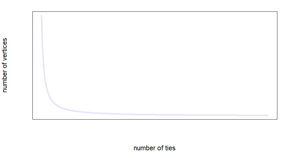

The “rich-get-richer” mechanism explains how hubs form in scale-free networks. Hubs are especially common in citation networks, biological systems, and technological networks, but not typically found in friendship or social networks, where humans have cognitive and temporal limits on the number of relationships they can maintain (Fuhse 2018).

To simulate scale-free networks, Barabási and Albert introduced a preferential attachment model for network growth. It starts with a small connected graph (e.g. two nodes with one edge) and then at each time step we add one more node and connect that node to an existing node \(i\) with probability:

\[\text{Prob(node i is chosen)}= \frac{deg(i)}{\sum_j deg(j)}\] This means nodes with higher degree are more likely to receive new edges, reinforcing hub formation.

The resulting degree distribution approximates a power law with expontne \(\gamma\) = 3.

Code

# Define number of vertices and edges
n <- vcount(karate)        # Number of vertices
total_edges <- ecount(karate)
m <- floor(total_edges / n)  # Approx. number of edges per node

# Generate preferential attachment graph
pa <- sample_pa(n = n,
                m = m,
                power = 2,
                directed = FALSE)
plot(pa, 
     vertex.color = "lavender")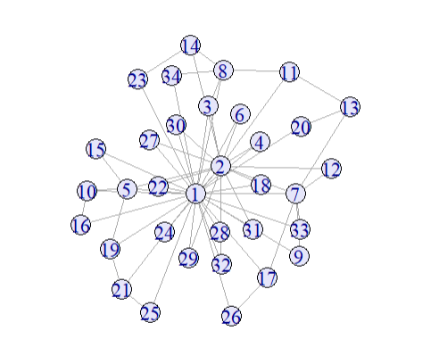

However, this simple process does not produce clustering (i.e., no triangles).

Exponential random graph models

Exponential Random Graph Models (ERGMs) are a powerful framework for modeling the structure of a single observed network. They allow us to quantify which types of configurations are statistically more or less likely than expected by chance.

Formally, an ERGM models the probability of observing a network \(y\) as:

\[ P_\theta(Y = y) = \frac{\exp(\theta^\top g(y))}{k(\theta)} \]

Where: - \(g(y)\) is a vector of network statistics (e.g., number of edges, triangles, degree counts), - \(\theta\) are model parameters, - \(k(\theta)\) is the normalizing constant (summing over all possible networks with the same node set).

They provide a statistical hypothesis test for network structure.
The fitted parameters tell us which features (e.g. triads, hubs, reciprocity) are present and significant.
We can simulate networks from the fitted model to compare other metrics (e.g., path lengths, clustering) to the observed network.

ERGMs are especially useful when we want to go beyond descriptive statistics and understand what social processes might be generating the observed structure.

Fitting ergms with `statnet`

The statnet suite provides a powerful set of tools for:

model estimation
model-based simulation
goodness-of-fit diagnostics

Following the ergm-tutorial of Chen (- Chen n.d.), We’ll use the flomarriage dataset: a historical network of marriage alliances among powerful families in Renaissance Florence .

Code

library(ergm)
data(package="ergm")
data(florentine)

class(flomarriage) #statnet networks are objects of class "network"

flomarriage

summary(flomarriage)

plot(flomarriage)

#Provide the statistics of the network
summary(flomarriage~edges+triangle)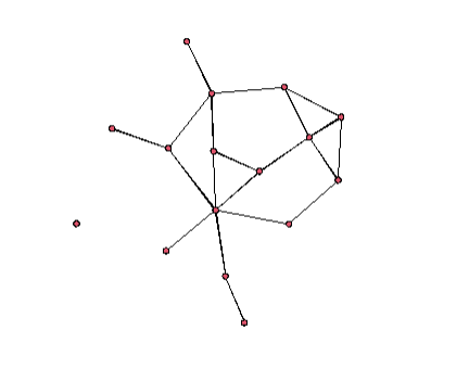

Specify network statistics

We can specify the network statistics \(g(y)\) to functions in the ergm package using the terms.

Most common terms are:

Name	Unit of Counting	Description	Num. of Statistics	Dep/Ind	Dir/Undir	Unip/Bip
edges	edges	Number of edges	1	ind	both	both
nodefactor	units of the attribute	Times nodes with a categorical attribute level appear in the edge set	1 per level	ind	both	both
nodematch	edges	Edges where incident nodes match on a nodal attribute	1 or per level	ind	both	both
nodemix	edges	Edges between combinations of nodal attribute values	1 per combination	ind	both	both
nodecov	units of the attribute	Sum of nodal attribute values for incident nodes across all edges	1	ind	both	both
absdiff	units of the attribute	Absolute difference in a nodal attribute between incident nodes	1	ind	both	both
mutual	dyad	Number of mutual edges (a → b and b → a)	1	dep	dir	both
degree	node	Number of nodes with degree x	1 per degree value	dep	undir	unip
idegree	node	Number of nodes with in-degree x	1 per degree value	dep	dir	unip
odegree	node	Number of nodes with out-degree x	1 per degree value	dep	dir	unip
b1degree	node	Number of mode 1 nodes with degree x	1 per degree value	dep	undir	bip
b2degree	node	Number of mode 2 nodes with degree x	1 per degree value	dep	undir	bip
mindegree	node	Number of nodes with at least degree x	1 per degree value	dep	undir	unip
triangles	triangles	Number of triangles	1 (more if attributes used)	dep	undir	unip
gwesp	complex	Geometrically weighted edgewise shared partners	1	dep	both	unip

For full list, in R type: help("ergm-terms")

When fitting an ergm we can think of ergm(y~x) as analogous to glm(y~x) - but for networks.

So these statistics make uup the \(g(y)\)-vector.

For example:

summary(flomarriage ~ edges + triangle + kstar(1:3) + degree(0:5))

edges: overall density
triangle: tendency toward triadic closure
kstar(1:3): centralization / popularity (2-stars, 3-stars, etc.)
degree(0:5): distribution of node degrees

We can start by fitting the most simple ergm (with only the edges term). This is similar to comparing networks to the Erdos-Renyi graphl, assuming there is no structure beyond density.

T(G) = #edges, = log

flomodel.01 <- ergm(flomarriage ~ edges)

# View model summary
summary(flomodel.01)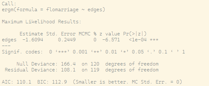

The interpretation is similiar to when you interpret glm:

edges Coefficient: If the coefficient is -1.6094, then: If the number of edges increase 1, the log-odds of an edge existing between any two nodes is -1.6094 -The probability of a tie between any two nodes is approximately 16.6%.
\(p< \alpha\): parameter does not equal to 0 significantly,
Null Deviance: The null deviance in the ergm output appears to be based on an Erdos-Renyi random graph with p = 0.5.
Residual Deviance: 2 times difference of loglik (saturated model - our model) (smaller is better)
AIC, BIC: loglik+penalty(#parameter)

Include `triangle` terms as a measure of clustering:

flomodel.02=ergm(flomarriage~edges+triangle)

summary(flomodel.02)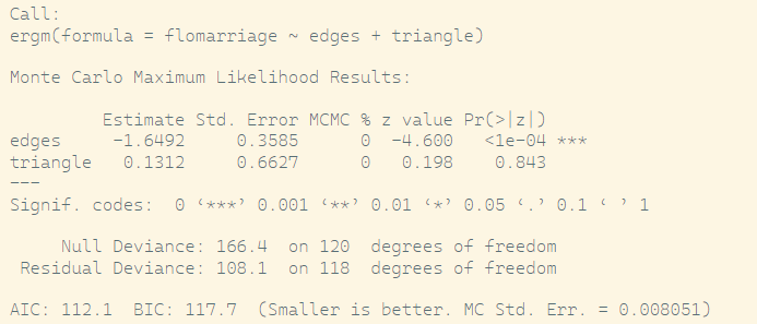

Include nodal covariates:

We can include continuous nodal covariates

Code

wealth=flomarriage %v% 'wealth' # %v% get the vertex attributes

plot(flomarriage, vertex.cex=wealth/25, main="Florentine marriage by wealth", cex.main=0.8)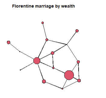

flomodel.03=ergm(flomarriage~edges+nodecov('wealth'))
summary(flomodel.03)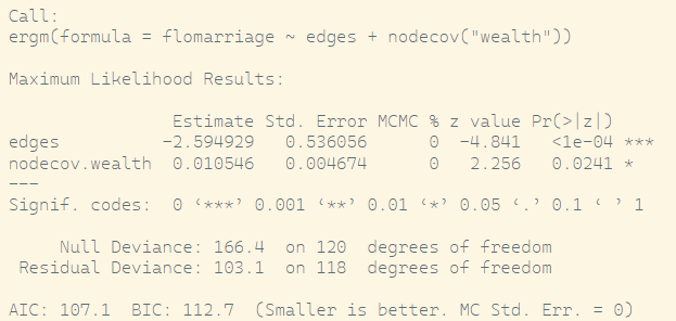

Baseline (edges):
The log-odds of a tie between two nodes with zero wealth is −2.595. This corresponds to a low baseline probability of a tie:

\[ \text{logit}^{-1}(-2.595) \approx 0.0695 \]

→ So, with no wealth effect, there’s about a 7% chance of a tie forming.

Wealth effect:

For each unit increase in wealth, the log-odds of a tie increase by 0.01055, per node. So:

If both nodes increase wealth by 1 unit, the log-odds of a tie increase by:

\[ 2 \cdot 0.01055 = 0.0211 \]

In probability terms, this is a small but positive effect:
→ Richer nodes are more likely to form ties, and the effect is additive across node pairs.

Include transformation of continuous nodal covariates:

Effect of absolute wealth difference: Specifically, it says:

“Are families with similar wealth more likely to form marriage ties?”

flomodel.04=ergm(flomarriage~edges+absdiff("wealth"))

summary(flomodel.04)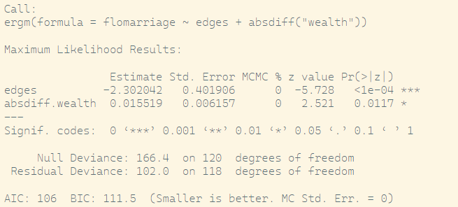

This is the baseline log-odds of a tie between two nodes, assuming their wealth is equal.
Translating to probability:

\[ \text{logit}^{-1}(-2.302) \approx \texttt{plogis(-2.302)} \approx 0.091 \]

→ So, when wealth difference is 0, there’s about a 9.1% chance of a tie.

Coefficient wealth difference:

This means for each unit increase in the absolute difference of wealth between two families, the log-odds of a tie increases by 0.0155.
This is counterintuitive — we would normally expect that greater wealth differences decrease tie probability. But here, ties are more likely as the difference grows.

→ Interpretation: Wealth difference may be associated with strategic marriages between wealthy and less wealthy families (e.g., alliances).

Code

plogis(-2.302 + 0.0155*5)

Include categorical (or discrete) variables

data("faux.mesa.high")
mesa=faux.mesa.high
mesa

fauxmodel.01=ergm(mesa ~edges + nodecov('Grade'))

summary(fauxmodel.01)

fauxmodel.02=ergm(mesa ~edges + nodefactor('Grade'))

summary(fauxmodel.02)

Include Homophily:

nodematch: Uniform homophily and differential homophily
uniform homophily(diff=FALSE), adds one network statistic to the model, which counts the number of edges (i,j) for which attrname(i)==attrname(j).
differential homophily(diff=TRUE), p(#of unique values of the attrname attribute) network statistics are added to the model.
The \(k\)th such statistic counts the number of edges \((i,j)\) for which attrname(i) == attrname(j) == value(k), where value(k) is the \(k\)th smallest unique value of the attrname attribute.
When multiple attribute names are given, the statistic counts only ties for which all of the attributes match.

Code

fauxmodel.03 <- ergm(mesa ~edges + nodematch('Grade',diff=F) )

summary(fauxmodel.03)

–> Nodes that share the same attribute are more likely to form a tie. –> Indicates homophily.

Code

fauxmodel.05 <- ergm(mesa ~edges + nodematch('Grade',diff=F)+ nodematch('Race',diff=T) )

summary(fauxmodel.05)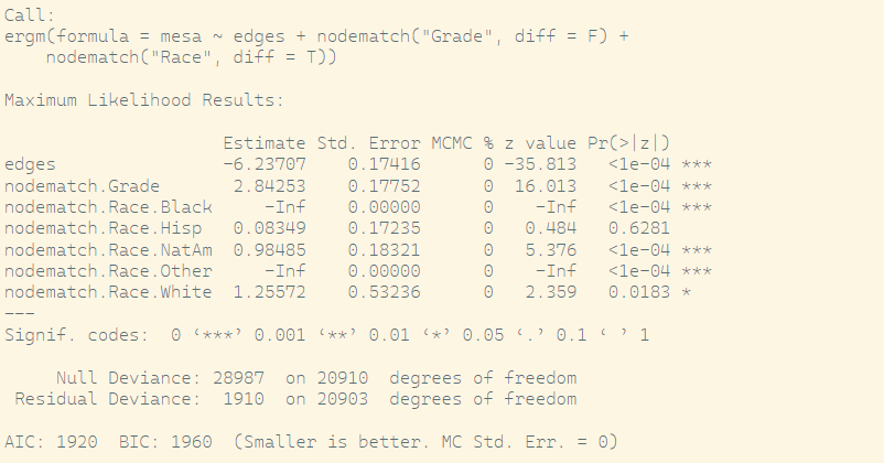

Simulation of networks using statnet

We can use models to similate other networks, maintaining the characteristics defined in the model.

Code

flomodel.04.sim <- simulate(flomodel.04, nsim=10,seed = 1)

summary(flomodel.04.sim)

Exercise:

Use the following code to load the karate network from the ìgraphdata package as an object of the network class.

Code

net <- asNetwork(karate)

Use ergms to answer these questions and interpret the results.

Are ties more likely to form between members of the same faction?

Is there evidence of triadic closure¹?

Stochastic Actor-Oriented Models (SAOMs) for longitudinal network analysis

We sadly do not have enough time to delve into these interesting analysis tools in the scope of this seminar but I still want to include them for completeness.

Stochastic Actor-Oriented Models (SAOMs) (Snijders, Van De Bunt, and Steglich 2010) are designed to capture the dynamic evolution of social networks by modeling the decisions and actions of individual actors over time. Unlike static network models, SAOMs incorporate an action-theoretic perspective, emphasizing that network changes result from intentional choices made by actors who seek to optimize their social positions according to certain preferences and constraints. This micro-level focus allows SAOMs to simulate how individual behavior drives the gradual transformation of the network structure, making them particularly well suited for analyzing longitudinal network data.

If you want to have a first look yourself: https://de.slideshare.net/slideshow/22-an-introduction-to-stochastic-actororiented-models-saom-or-siena/175668810 and https://www.stats.ox.ac.uk/~snijders/siena/IntroSAOM_h.pdf here are a straightforward introductions.

—

Insights from Network-Studies

To sum things up on our knowledge on social network analysis and in order to get inspired on what we actually can do with these tools now, that we have learned so much, I have collected some case studies from the literature and some insights that they provide us with: Lets start with one, that we have already looked at today:

Power in Rennaissance Florence (Padgett and Ansell 1993)

Code

name=flomarriage %v% 'vertex.names'

plot(flomarriage,
     vertex.cex=wealth/25,
     main="Florentine marriage by wealth",
     cex.main=0.8,
     label = name,
     vertex.col="lavender")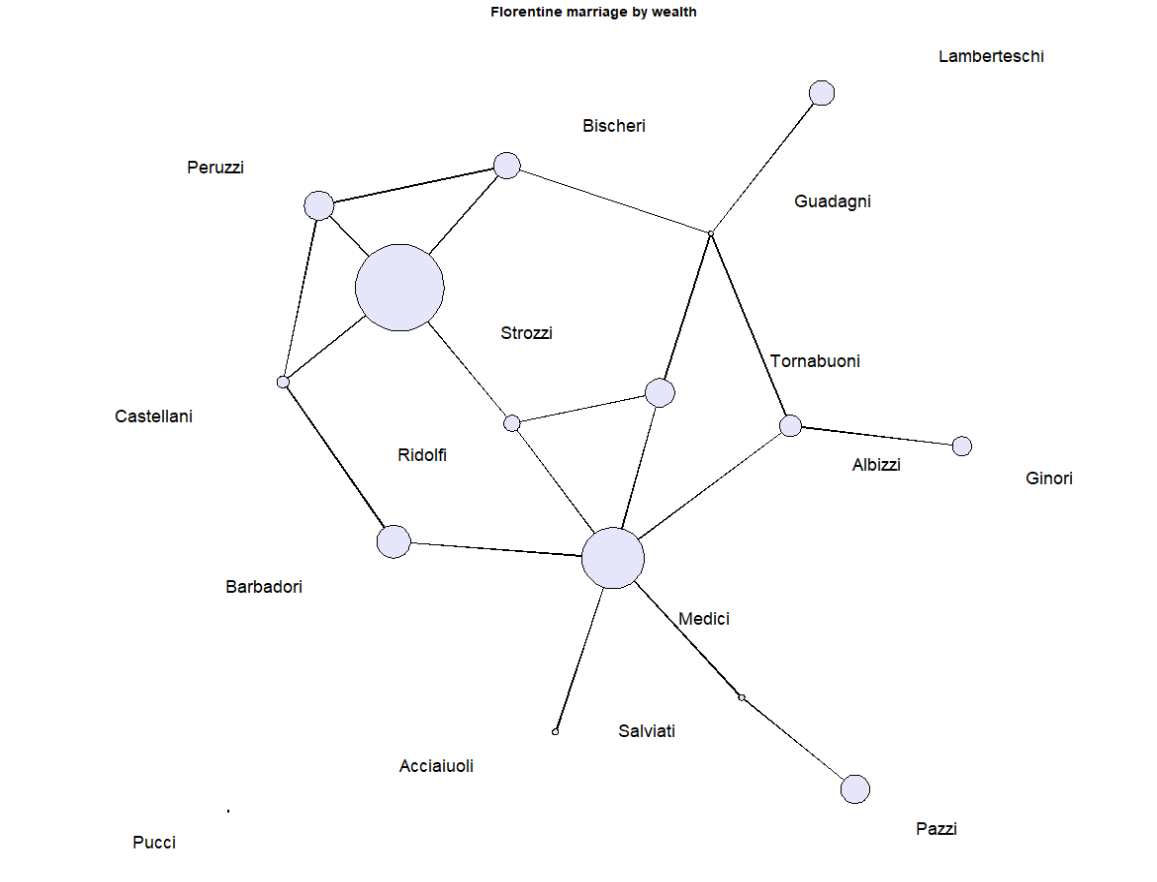

The Florentine marriage network offers a compelling demonstration of how network structure can reveal the foundations of social and political power. Although the Medici family began with relatively modest wealth and political influence, Cosimo de’ Medici strategically leveraged intermarriage ties, economic relationships, and political patronage to consolidate power. His actions positioned the Medici as central brokers within Florence’s elite social network.

While other families like the Strozzi possessed greater wealth and held more political offices, they lacked the Medici’s structural advantage. A simple count of marriage ties shows the Medici ahead—but only marginally. However, a deeper look using betweenness centrality reveals their unique position: the Medici were on over half of all shortest paths connecting other families in the network, with a betweenness score of 0.522. In contrast, the Strozzi scored just 0.103, and the next most central family, the Guadagni, scored 0.255.

This measure reflects the Medici’s pivotal role in brokering connections across elite families. For example, the Medici connected the Barbadori and Guadagni via multiple shortest paths, acting as a key intermediary. Such centrality enabled them to influence communication, marriage arrangements, business alliances, and political decisions.

These findings show how network structure provides critical insight beyond wealth or formal political power. It demonstrates that:

Influence often stems from positional advantage within a network rather than from resources alone.
Betweenness centrality can uncover hidden forms of power—especially brokerage roles.
Social alliances (like marriages) were consciously used by patriarchs to shape political landscapes.
The Medici capitalized on structural gaps or “disjunctures” in the elite network—opportunities that others failed to exploit.

As Padgett and Ansell note, Medician control emerged not from dominance in wealth or titles, but from bridging divides among rival families — something only the Medici managed to achieve. This suggests that elite social networks were both instruments and outcomes of intentional strategy.

The Frog-Pond Effect (Frank 1985)

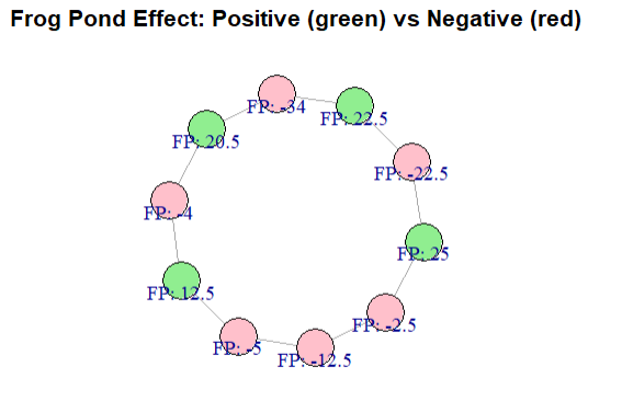
The Frog Pond Effect describes how individuals assess their own abilities not in absolute terms, but relative to those around them. In other words, whether someone feels successful or competent depends heavily on the context or “pond” they’re in.

Being a “big frog in a small pond” — for instance, a strong performer in a weak peer group—often leads to higher self-esteem, while being a “small frog in a big pond” can lead to feelings of inadequacy, even if one’s actual performance is the same.

In network terms:

Each person (node) compares themselves mainly to their local neighborhood (connected peers).
The structure of the social network can therefore influence how individuals perceive their own status or competence.
For example, a student with average grades might feel very different about their performance depending on whether their friends are mostly top students or struggling ones.

This has important implications:

Self-perception and motivation are not purely personal traits—they are shaped by the immediate social context.
In educational settings or workplaces, the composition of peer groups can affect confidence and behavior, even without changing actual outcomes.

g <- make_ring(10) %>%
  set_vertex_attr("name", value = LETTERS[1:10]) %>%
  set_vertex_attr("achievement", value = c(85, 90, 70, 60, 75, 95, 65, 80, 50, 88))

# Function to calculate frog pond effect for each node
frog_pond <- function(graph) {
  ego_scores <- numeric(vcount(graph))
  for (i in V(graph)) {
    neighbors <- neighbors(graph, i)
    if (length(neighbors) > 0) {
      avg_neighbor <- mean(V(graph)[neighbors]$achievement)
      ego_scores[i] <- V(graph)[i]$achievement - avg_neighbor
    } else {
      ego_scores[i] <- NA  # No neighbors
    }
  }
  return(ego_scores)
}

# Calculate effect and add as attribute
V(g)$frogpond <- frog_pond(g)

# Visualize the graph
plot(
  g,
  vertex.size = 30,
  vertex.label = paste0("\nFP: ", round(V(g)$frogpond, 1)),
  vertex.color = ifelse(V(g)$frogpond > 0, "lightgreen", "pink"),
  main = "Frog Pond Effect: Positive (green) vs Negative (red)"
)

Why your friends have more friends than you do (Feld 1991)

The Friendship Paradox reveals a surprising social network property:

“On average, your friends have more friends than you do.”

This paradox arises due to how degree centrality interacts with the network structure: individuals with more friends are more likely to appear in others’ friend lists, which biases the average.

Code

# Create a small example network

g <- sample_pa(20, p = 0.2, directed = FALSE)

if (is.null(V(g)$name)) {
  V(g)$name <- as.character(seq_along(V(g)) - 1)  # igraph uses 0-based indexing
}


# Get the degree (number of friends) for each node
degree_values <- igraph::degree(g)

# For each node, compute the average degree of their neighbors
friend_avg_degrees <- sapply(V(g), function(v) {
  neighbors_v <- neighbors(g, v)
  if (length(neighbors_v) == 0) return(NA)
  mean(igraph::degree(g, neighbors_v))
})

# Compare own degree to the average degree of neighbors
comparison_df <- data.frame(
  node = V(g)$name,
  own_degree = degree_values,
  friends_avg_degree = friend_avg_degrees,
  paradox = friend_avg_degrees > degree_values
)

# Output summary
print(comparison_df)

# Optional: visualize who experiences the paradox
V(g)$color <- ifelse(friend_avg_degrees > degree_values, "orange", "lightblue")
plot(g, vertex.label = NA, vertex.size = 10, main = "Friendship paradox: Neighbours have higher degree (orange) vs Neighbours have lower degree (blue)")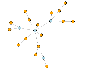

Friendship paradox: average degree of neighbour higher > i: orange, lower: blue

This ist’t just a statistical curiosity but has social consequences:

People may feel less popular or connected than average, even if they aren’t
It reflects sampling bias: highly connected nodes are more likely to appear in your local network.

Friendship and Romances among High School Students (Bearman, Moody, and Stovel 2004)

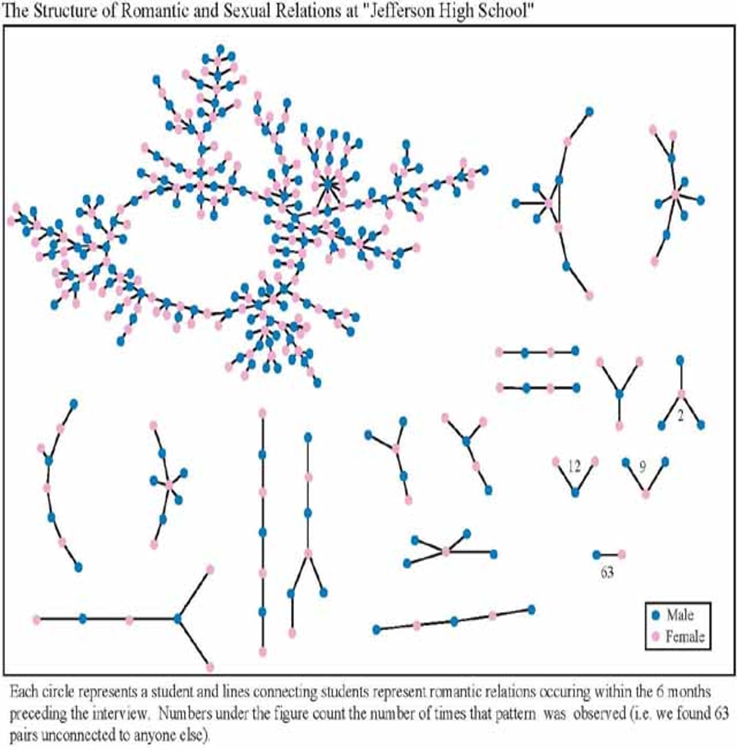
Bearman et al. (2004) asked which structural properties of social networks are relevant for the spread of diseases, as ego-centered network studies reveal little about the broader network structures that facilitate disease transmission. So in 1994 they conducted a study at a U.S. highschool (Jefferson High) with 832 students surveyed on their health status and their sexual and romantic partners in the past 8 months.

Network Characteristics
- Structure: Resembles a spanning tree
  - Chain-like network with minimal cycles
  - Very few closed loops (no cycle of length 4)
  - A small number of nodes serve as central connectors
- Size and Connectivity
  - 52% of students were in the largest connected component
  - Longest path within the largest component: 37 nodes
- Normative Influence
  - Network likely shaped by social norms limiting simultaneous partnerships
Key Insight
- The largest component is described as a “worst-case scenario for the potential transmission of disease” (Bearman, Moody, and Stovel 2004, 59)
- Most individuals had only one partner, yet due to the structure, their risk of infection was higher than those in isolated dyads or small clusters
Conclusion
- STD risk is not merely a function of partner count
  - Structural position within the network strongly affects exposure and vulnerability

In the network of the conclave (“In the Network of the Conclave - Bocconi University” 2025)²

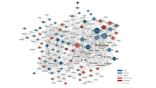
The study by Giuseppe Soda, Alessandro Iorio, and Leonardo Rizzo from Bocconi University explores how network science can shed light on the complex social, political, and relational dynamics behind the election of a new Pope. Although the final decision is traditionally attributed to divine inspiration, the researchers demonstrate that the structure of relationships within the College of Cardinals plays a crucial role in shaping consensus and influence.

Behind the closed doors of the Sistine Chapel, the papal election resembles the selection processes found in other organizational contexts—such as presidential elections or CEO appointments—yet it remains deeply embedded in ancient traditions and rituals. By mapping the Vatican as a relational ecosystem, the study identifies key factors that determine which cardinals are more likely to emerge as leading candidates, or papabili.

The researchers constructed a multi-layered network based on:

Official co-memberships: Connections through shared work in Roman Curia dicasteries, commissions, councils, and academies.
Episcopal consecrations: “Spiritual genealogies” that link cardinals through ordination and build loyalty.
Informal relationships: Ideological affinities, mentoring, and patronage networks revealed by journalistic sources.

These layers combined give a systemic map of the College of Cardinals, capturing formal and informal ties alike.

The study identifies three main criteria that increase a cardinal’s prominence in the network:

Status (Eigenvector Centrality): Reflects connections to influential cardinals, rewarding those linked to the most central figures.
Information Control (Betweenness Centrality): Highlights cardinals who serve as bridges or hubs between different groups.
Coalition Building Capacity: A composite measure capturing cohesion within groups, direct influence (number of connections), and the strategic role as a social broker linking different factions.

An additional factor is age, adjusted based on historical papal election trends favoring candidates of moderate age.

Top Status: Robert Prevost (US), Lazzaro You Heung-sik (South Korea), Arthur Roche (UK), Jean-Marc Aveline (France), Claudio Gugerotti (Italy) - Top Information Controllers: Anders Arborelius (Sweden), Pietro Parolin (Italy), Víctor Fernández (Argentina), Gérald Lacroix (Canada), Joseph Tobin (USA) - Top Coalition Builders: Luis Antonio Tagle (Philippines), Ángel Fernández Artime (Spain), Gérald Lacroix (Canada), Fridolin Besungu (Congo), Sérgio da Rocha (Brazil)

The network shows a strong presence of “soft liberal” cardinals and an increasingly global geographical spread, especially with growing roles for Asia and Africa.

It underscores several important insights for network theory:

Multi-layer networks: Combining formal, informal, and historical relational data provides a richer, more accurate representation of influence dynamics.
Centrality measures matter: Different types of centrality capture distinct aspects of power—status, information brokerage, and coalition-building.
Relational structures shape outcomes: Even in highly ritualized and spiritual processes, human relationships and social capital influence decisions.
Predictive yet humble modeling: While models can’t fully predict outcomes, they improve understanding of complex social phenomena.

Spread of happyness (Fowler and Christakis 2008)

The study investigates whether happiness spreads through social networks and whether distinct clusters of happy and unhappy individuals form within these networks. Previous research has focused on the role of socioeconomic and genetic factors in determining happiness, but this research takes a relational perspective, exploring how interpersonal connections influence emotional well-being over time.

Using a longitudinal dataset from the Framingham Heart Study, which tracked 4,739 individuals in Massachusetts between 1983 and 2003, the researchers applied social network analysis methods to explore the contagiousness of happiness. Happiness was measured using a validated four-item scale, providing a reliable metric of emotional well-being.

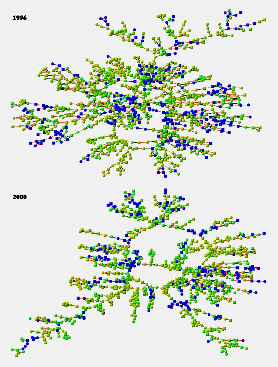
Happiness clusters in the Framingham social network. Graphs show largest component of friends, spouses, and siblings at exam 6 (centred on year 1996, showing 1181 individuals) and exam 7 (year 2000, showing 1020 individuals). Each node represents one person (circles are female, squares are male). Lines between nodes indicate relationship (black for siblings, red for friends and spouses). Node colour denotes mean happiness of ego and all directly connected (distance 1) alters, with blue shades indicating least happy and yellow shades indicating most happy (shades of green are intermediate)

The key findings were:

Existence of Clusters: Networks show distinct clusters of happy and unhappy people, supporting the idea of emotional homophily and influence.
Social Contagion: Individuals surrounded by many happy people have a significantly higher likelihood of being happy themselves.
Influence of Relationship Types: Contagion effects are strongest among friends, family members, neighbors, and spouses, but not among coworkers.
Network effects independently exist: Effects persist even after controlling for confounding factors such as shared environment and socioeconomic similarities.

With implications for sociology:

Emotional Contagion in Networks: Happiness spreads through social ties, highlighting the importance of network structure in shaping individual well-being.
Clusters as Emotional Ecosystems: Networks are not random but organize into niches or clusters of similar emotional states, reinforcing the idea of social reinforcement and peer effects.
Tie Strength and Type Matter: The differential impact of relationship types emphasizes the role of close and stable ties in transmitting emotions, while more formal or less intimate ties (e.g., coworkers) show weaker or no contagion effects.
Longitudinal Approach: Following actors over time allows for stronger causal inference about social influence beyond mere correlation or selection.

(Hashtag-homophily)

In my master’s thesis, I conduct a descriptive study on opinion homophily on Twitter. The motivation behind this research is that strong homophily — the tendency for people to connect with others who share similar beliefs — can lead to so called echo chambers and disrupt the broader societal discourse.

So I had a descriptive look following the question: To what extent do people connect (and disconnect) on Twitter based on similar opinions and convictions?

A friend of mine and I collected data (in a different seminar) on tweets on Twitter related to the hashtag #FridaysForFuture (e.g. Tweets, Account ID and Follower/Followee information on all tweets posted in the week between December 4th and December 10th 2019)

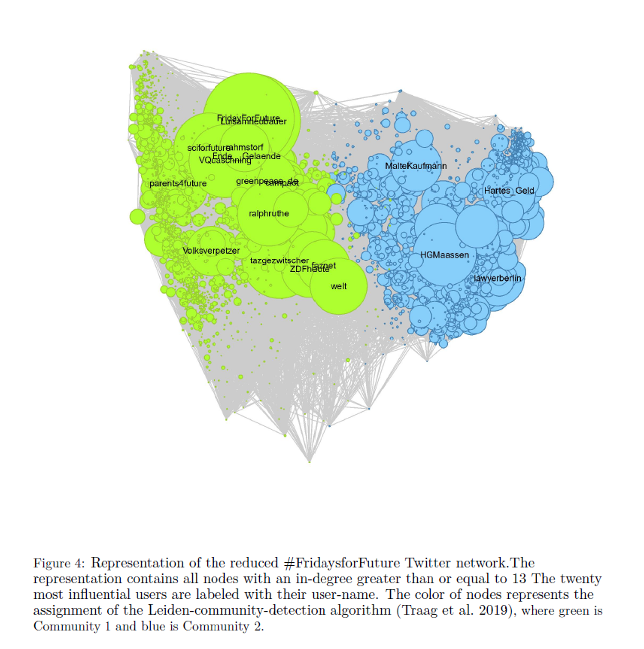
Descriptive comparison of communities:

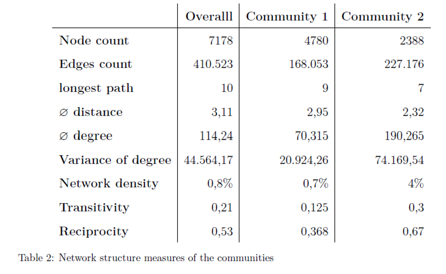
Comparison of discourse I then compared the content of the tweets by analyzing frequencies, emojis, and sentiment to determine whether the discourse differed significantly within each cluster. To be fair, today I wouldn’t use these same methods - which is fair, considering there were less chances to learn CSS methods when I studied 😅

References

Balasundaram, Balabhaskar, Sergiy Butenko, and Illya V. Hicks. 2011. “Clique Relaxations in Social Network Analysis: The Maximum k -Plex Problem.” Operations Research 59 (1): 133–42. https://doi.org/10.1287/opre.1100.0851.

Batagelj, V., and M. Zaversnik. 2003. “An O(m) Algorithm for Cores Decomposition of Networks.” arXiv. https://doi.org/10.48550/arXiv.cs/0310049.

Bearman, Peter S., James Moody, and Katherine Stovel. 2004. “Chains of Affection: The Structure of Adolescent Romantic and Sexual Networks.” American Journal of Sociology 110 (1): 44–91. https://doi.org/10.1086/386272.

Chen, Yunran. n.d. Chapter 3 ERGM (Statnet Package) Introduction to Network Analysis Using R. Accessed May 18, 2025.

Erdős, P., and A. Rényi. 1959. “On Random Graphs. I.” Publicationes Mathematicae Debrecen 6 (3-4): 290–97. https://doi.org/10.5486/PMD.1959.6.3-4.12.

Feld, Scott L. 1991. “Why Your Friends Have More Friends Than You Do.” American Journal of Sociology 96 (6): 1464–77. https://www.jstor.org/stable/2781907.

Fowler, J. H, and N. A Christakis. 2008. “Dynamic Spread of Happiness in a Large Social Network: Longitudinal Analysis over 20 Years in the Framingham Heart Study.” BMJ 337 (dec04 2): a2338–38. https://doi.org/10.1136/bmj.a2338.

Frank, Robert H. 1985. Choosing the Right Pond : Human Behavior and the Quest for Status. New York ; Oxford [Oxfordshire] : Oxford University Press.

Fuhse, Jan. 2018. Soziale Netzwerke: Konzepte und Forschungsmethoden. 2., überarbeitete Auflage. UTB Sozialwissenschaften 4563. Konstanz: UVK Verlagsgesellschaft mbH. https://doi.org/10.36198/9783838549811.

“In the Network of the Conclave - Bocconi University.” 2025. https://www.unibocconi.it/en/news/network-conclave.

Kolaczyk, Eric D., and Gábor Csárdi. 2020. Statistical Analysis of Network Data with R. Second Edition 2020. Cham: Springer.

Newman, M. E. J. 2004. “Detecting Community Structure in Networks.” The European Physical Journal B - Condensed Matter 38 (2): 321–30. https://doi.org/10.1140/epjb/e2004-00124-y.

Nutarelli, Federico. 2024. “A Quick Look to Louvain Clustering.” Federico Nutarelli. https://www.federiconutarelliphd.com/post/a-quick-look-to-louvain-clustering.

Padgett, John F., and Christopher K. Ansell. 1993. “Robust Action and the Rise of the Medici, 1400-1434.” American Journal of Sociology 98 (6): 1259–319. https://doi.org/10.1086/230190.

Smith, Chris M., and Andrew V. Papachristos. 2021. “Criminal Networks.” In The Oxford Handbook of Social Networks, edited by Ryan Light and James Moody, 0. Oxford University Press. https://doi.org/10.1093/oxfordhb/9780190251765.013.37.

Snijders, Tom A. B., Gerhard G. Van De Bunt, and Christian E. G. Steglich. 2010. “Introduction to Stochastic Actor-Based Models for Network Dynamics.” Social Networks 32 (1): 44–60. https://doi.org/10.1016/j.socnet.2009.02.004.

Zachary, Wayne W. 1977. “An Information Flow Model for Conflict and Fission in Small Groups.” Journal of Anthropological Research 33 (4): 452–73. https://doi.org/10.1086/jar.33.4.3629752.

Footnotes

Including a triangle term can lead to overfitting in small networks, so it might generally better to use the gwesp() term instead. This term captures triadic closure in a more stable way by applying a geometrically weighted decay to the count of shared partners for each edge.↩︎
The official paper is not yet published↩︎

Why study social groups?

Basic subgroup concepts

Cliques

n-Cliques

k-Core Subgraphs

K-Plex subgraphs

Cohesive groups

Community detection algorithms

Communities via edge betweenness

The Girvan-Newman Method

Modularity based

Fast and Greedy Algorithm

Louvain

Leiden

Further community detection algorithms implemented in igraph

Getting community information

Validation of Community

—

Network inference

Model-Free Simulation (Null Random Graphs)

Bernoulli (Erdós-Renyi) Random graphs

The Barabasi-Albert model

Exponential random graph models

Fitting ergms with statnet

Specify network statistics

Include triangle terms as a measure of clustering:

Include nodal covariates:

Include transformation of continuous nodal covariates:

Include categorical (or discrete) variables

Include Homophily:

Simulation of networks using statnet

Stochastic Actor-Oriented Models (SAOMs) for longitudinal network analysis

—

Insights from Network-Studies

Power in Rennaissance Florence (Padgett and Ansell 1993)

The Frog-Pond Effect (Frank 1985)

Why your friends have more friends than you do (Feld 1991)

Friendship and Romances among High School Students (Bearman, Moody, and Stovel 2004)

In the network of the conclave (“In the Network of the Conclave - Bocconi University” 2025)2

Spread of happyness (Fowler and Christakis 2008)

(Hashtag-homophily)

References

Footnotes

Copyright

Further community detection algorithms implemented in `igraph`

Fitting ergms with `statnet`

Include `triangle` terms as a measure of clustering:

In the network of the conclave (“In the Network of the Conclave - Bocconi University” 2025)²