Code
library(needs)
needs(igraph,
      ggraph,
      ggplot2,
      patchwork)

# Set seed for reproducibility
set.seed(123)Welcome to the second session of the seminar Computational Social Sciences
library(needs)
needs(igraph,
ggraph,
ggplot2,
patchwork)
# Set seed for reproducibility
set.seed(123)In the context of social network analysis from a sociological perspective, we typically discuss two broad aspects.
One of these aspects revolves around network theories, which explore how individuals behave within social contexts and how networks themselves evolve and function. Central questions in this area include: Where do network relationships originate? How are they formed? And what are the implications and consequences of these relationships for the people involved (Lizardo and Isaac Jilbert 2023)
Reflect briefly on the occasions, where in the past you have been confronted with social networks theories. In what theoretical concepts of sociology is the embedding of actors of central importance?
The other big branch focuses mostly on the description of networks and on how to measure various network properties. It links social network contexts to a quantitative representation.
In this class we will try to have a look at both “faces” of social network analysis. We will learn some of the basic concepts and how they connect to measurable network properties.
Imagine you were to plot all relationships of all people in the world. Of course, this is just not possible, as the measurement but also the representation would be too complex. Thus we need some kind of (theoretical) bounds, that make the analysis of networks possible.
In social network analysis, we use graphs to represent social networks. We borrow graphs from the mathematical graph theory which also provides us with a definition (Joshi 2017).
A graph \(G\) consists of a vertex set \(V\) and an edge set \(E\):
\[ G = \{V, E\} \]
where \(V\) is a set of nodes \(V=\{v_1,v_2,v_3\}\) and \(E\) being a set of edges \(E = \{\{v_1,v_2\},\{v_2,v_3\}\}\).
By using set theory, we can rigorously define different types of graphs, operations on graphs, and concepts like subgraphs, neighbourhoods, or connectivity.
Short Digression: Set Theory
Sets are collections of distinct elements. The order and repitition of elements in a set does not matter.
| Symbol | Usage | Interpretation in Graphs |
|---|---|---|
| \(\emptyset\) | \(\{\}\) | Empty set (e.g., a graph with no edges) |
| \(\cup\) | \(A \cup B\) | Union of sets (e.g., merging vertex or edge sets) |
| \(\cap\) | \(A \cap B\) | Intersection of sets (e.g., common neighbors) |
| \(\setminus\) | \(A \setminus B\) | Set difference (e.g., removing edges or vertices) |
| \(\times\) | \(A \times B\) | Cartesian product (e.g., possible edge pairs in a complete graph) |
| \(\mathfrak{P}()\) | \(\mathfrak{P}(A)\) | Power set (e.g., all possible subsets of vertices or edges) |
| \(\subset\) | \(A \subset B\) | Subset (e.g., a subgraph is a subset of a larger graph) |
| \(\in\) | \(x \in A\) | Element in a set (e.g., a vertex in a vertex set) |
| \(\notin\) | \(x \notin A\) | Element not in a set (e.g., a missing edge in a sparse graph) |
In social network analysis, we distinguish between directed and undirected networks. In most real-world cases, directed networks are more realistic because relationships are often asymmetric. However, undirected networks are easier to analyze mathematically and computationally.
Directed networks represent relationships where the connection has a defined direction. These relationships do not necessarily have to be reciprocal.
\[ \forall A,B \in V:(A \to B) \not\Rightarrow (B \to A) \]
Examples:
- Social media interactions: On Twitter or Instagram, one user can follow another without being followed back.
- Communication networks: E-Mails, phone calls or other forms of communication, can be sent out or received, thus defining a direction.
Note: In a directed graph, the edges are ordered, meaning the edge ( (a, b) ) is not the same as ( (b, a) ). The direction of the edge matters, and there is a one-way connection from ( a ) to ( b ) (but not necessarily the other way around).
Edges in directed graphs are thus representations of ordered pairs (tuples). We can write these as \(E = \{(a,b), (b, c), (c, d), (d, a)\}\).
Undirected networks assume that if a connection exists, it is inherently mutual. These networks are simpler to analyze since they do not require considering directionality.
\[ \forall A, B \in V: (A \leftrightarrow B) \Rightarrow (B \leftrightarrow A) \]
Examples:
- Mutual friendships: In many studies, friendship networks are assumed to be undirected, meaning if A considers B a friend, B also considers A a friend (although this is not always the case in reality).
- Co-authorship networks: If two researchers have co-authored a paper together, the connection exists for both equally.
- Collaboration networks: In corporate or scientific collaborations, individuals or institutions work together on projects, making the relationship inherently bidirectional. - Classmates
Note: In an undirected graph, the edges are unordered, meaning the edge ( {a, b} ) is the same as ( {b, a} ). The connection between ( a ) and ( b ) has no direction, and this is reflected by the use of unordered pairs in the edge set.
A graph \(E\) where there are no multiple edges and where each edge is an unordered pair \({a,b}\) with \(a /neq b\) is also called a simple graph$
In practice, the choice between directed and undirected networks depends on the research question. If directionality is crucial (e.g., influence, hierarchy, or information flow), a directed network is necessary. However, if the goal is to analyze overall connectivity, undirected networks provide a simpler approach.
# Generate a random graph with 30 nodes and 50 edges
g2 <- sample_gnm(n = 60, m = 70,  directed = TRUE)

# Assign random colors to nodes
V(g2)$color <- sample(c("blue", "green"), vcount(g2), replace = TRUE)

# Assign random sizes to nodes
V(g2)$size <- sample(5:12, vcount(g2), replace = TRUE)

  # Plot the network using ggraph
p1 <- ggraph(g, layout = "fr") +
      geom_edge_link(color = "gray", alpha = 0.5) +
      geom_node_point(aes(size = size, color = color), alpha = 0.8) +
      scale_color_manual(values = c("blue" = "#967bb6", "green" = "#e8bff7")) +
      theme_void() +
      theme(legend.position = "none") +
      ggtitle("Undirected Network")

# Create the directed network plot
p2 <- ggraph(g2, layout = "fr") +
  geom_edge_link(arrow = arrow(length = unit(1.8, "mm"), type = "closed"), color = "gray", alpha = 0.3) +
  geom_node_point(aes(size = size, color = color), alpha = 0.8) +
  scale_color_manual(values = c("blue" = "#967bb6", "green" = "#e8bff7")) +
  theme_void() +
  theme(legend.position = "none") +
  ggtitle("Directed Network")

# Combine the plots
combined_plot <- p1 + p2

# Save as PNG
ggsave("Graphics/undirected_directed.png", plot = combined_plot, width = 15, height = 6, dpi = 300)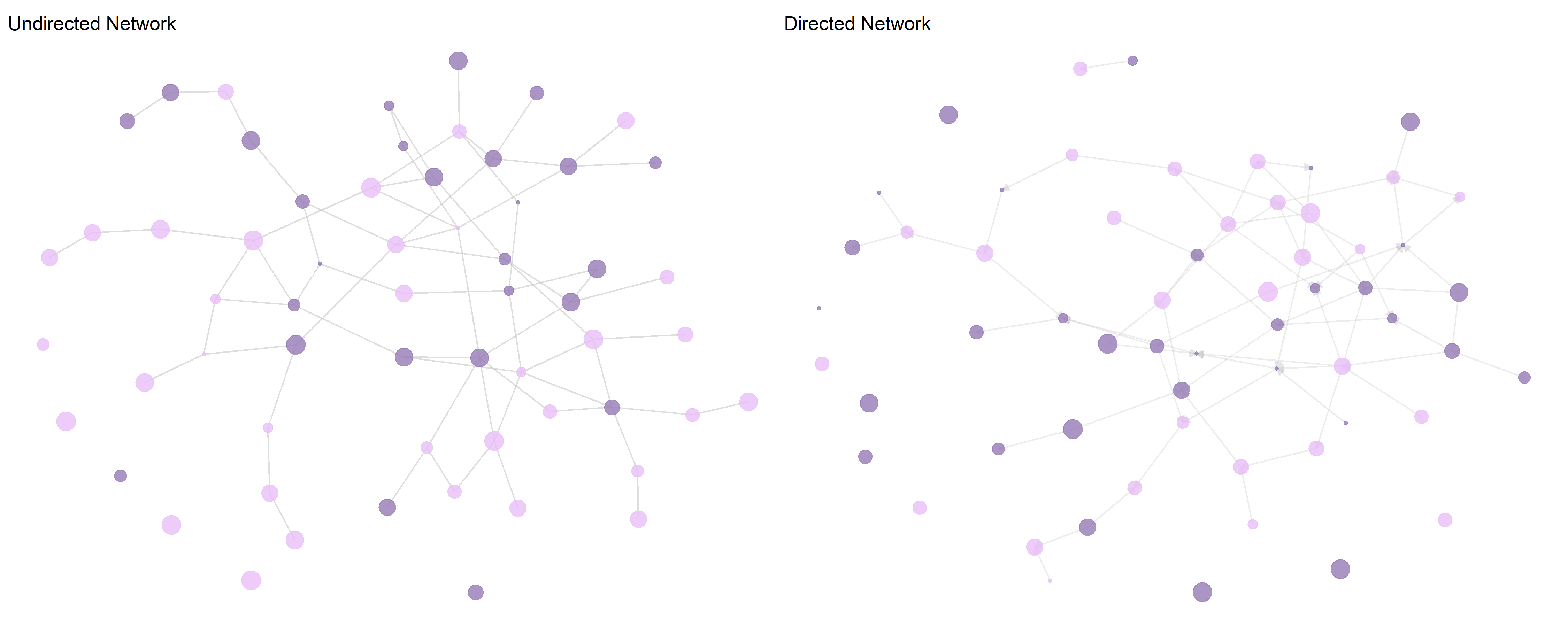
In academic research, networks are often represented as graphs. For small datasets, this visualization is quite intuitive. A quick glance at such a diagram can give us a good sense of the network’s structure.
However, as networks grow larger, this representation quickly reaches its limits. With hundreds, thousands, or even millions of nodes and edges, we end up with what network analysts call a “hairball”—a dense, tangled structure from which little insight can be gained.
This is why, alongside graphical representations, there are other, mathematically more powerful approaches. While they may seem less intuitive, they allow for precise calculations and the analysis of large networks. While graphs help us visually grasp networks, matrices or edge lists serve as the essential tools for conducting complex computations in network analysis.
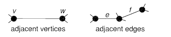
Adjacency: We say that two vertices \(v\) and \(w\) of a graph \(G\) are adjacent if there is an edge joining them, and the vertices v and w are then incident with such an edge. Similarly, two distinct edges \(e\) and \(f\) are adjacent if they have a vertex in common (Wilson 2009).
To analyze large networks effectively, we often use adjacency matrices. An adjacency matrix \(A\) is a square matrix used to represent a finite graph. Each row and column correspond to a node in a network. The entries of the matrix indicate whether a connection exists between two nodes.
In the simplest form, the matrix contains binary values:
\[ A = (A_{ij})_{i,j \in V},\text{ where } A_{ij} = \begin{cases} 1, & \text{if there is an edge between node } i \text{ and node } j \\ 0, & \text{otherwise} \end{cases} \]
Diagonal elements: \(A_{ii}\) is typically 0 because a node is not connected to itself.
For an undirected graph, the adjacency matrix is symmetric, meaning \(A_{ij} = A_{ji}\). In contrast, for a directed graph, the matrix is generally asymmetric, where \(A_{ij} = 1\) indicates a directed edge from node \(i\) to node \(j\), but not necessarily vice versa.

By using different values than 0 and 1 in \(A\) , we can also represent a weight of a connection (e.g strength of a friendship, the frequency of interaction or any other meaningful measure of connection intensity).
Similiarly to the adjacency matrix a adjacency list stores the information if one node in a graph is connected to another, while being a lot more space efficient.
An adjacency list is a collection of lists, where each node has a list of its neighbours.
We can convert from an adjacency matrix to a adjacency list in the way that we iterate over the matrix \(A\) and for each entry \(A_{ij} = 1\), we add node \(j\) to the adjacency list of node \(i\).
| directed | undirected | |
|---|---|---|
| 1 | (4,7) | (4,6,7) |
| 2 | (3,7) | (3,5,7) |
| 3 | (2,6) | (2,4,6) |
| 4 | (1,3) | (1,3,5) |
| 5 | (2,4,7) | (2,4,6,7) |
| 6 | (1,3,5) | (1,3,5,7) |
| 7 | () | (1,2,5,6) |
With even bigger networks it might be useful to even store networks in an edge list, where each edge is represented as a pair (or triplet in weighted graphs) indicating a connection between two nodes.
| directed | undirected | |
|---|---|---|
| V | 1, 2, 3, 4, 5, 6, 7 | 1, 2, 3, 4, 5, 6, 7 |
| E | (1,4), (1,7), (2,3), (2,7), (3,2), (3,6), (4,1), (4,3), (5,2), (5,4), (5,7), (6,1), (6,3), (6,5) | {1,4}, {1,6}, {1,7}, {2,3}, {2,5}, {2,7}, {3,4}, {3,6}, {4,5}, {5,6}, {5,7}, {6,7} |
Tip:
igraph objectsIn igraph (Csárdi et al. 2025), a network object is an instance of the class igraph. There are multiple ways to create such an object, depending on the available data format:
graph_from_literal(): Allows for quick creation of small graphs using a formula-like syntax.
graph_from_adj_list(): Generates a graph from an adjacency list.
graph_from_edgelist(): Constructs a graph from an edgelist.
graph_from_adjacency_matrix(): Builds a graph from an adjacency matrix.
read_graph():Reads graphs from various file formats, including GraphML and Pajek.
graph_from_data_frame(): Creates a graph from data frames containing edge lists and optional vertex attributes. This is the preferred method for importing tabular data.
Directed graph:
M <- matrix(c( 0, 1, 0, 0, 0,
               0, 0, 1, 0, 0,
               1, 1, 0, 0, 1,
               0, 1, 0, 0, 0,
               0, 1, 1, 0, 0), nrow = 5, byrow=TRUE)

g <- graph_from_adjacency_matrix(M, mode = "directed")

# Graph descriptives
summary(g)

V(g)  # List nodes
E(g)  # List edges

as_edgelist(g)  # Convert to edge list
as_adjacency_matrix(g) # Get adjacency matrix
as_adj_list(g, mode = "out") # Get adjacency list

vcount(g)  # Count vertices
ecount(g)  # Count edges

# Plot the graph
plot(g)
Undirected graph:
ug <- graph_from_adjacency_matrix(M, mode = "max") # max nimmt für jeden Kante den größeren Wert (i,j), (j,i)
ug
summary(ug)

V(ug)
E(ug)

as_edgelist(ug)
as_adjacency_matrix(ug)
as_adj_list(ug, mode = "out")

vcount(ug)
ecount(ug)

plot(ug)
Accessing the Adjacency matrix
as_adjacency_matrix(g)  # Retrieve adjacency matrix
g[]  # Print entire adjacency matrix
g[2,1]  # Check if an edge exists from node 2 to 1
g[1,2]  # Check edge from node 1 to 2
g[2,]   # Get all edges originating from node 2
sum(g[2,]) # Count outgoing connections from node 2edgelist <- rbind(c(1,2), c(1,3), c(2,3), c(2,4), c(3,2), c(5,3))
h <- graph_from_edgelist(edgelist)
plot(h)g <- graph_from_literal(1--2, 2--3, 3--5, 4--2, 1--3, 2--5)
plot(g)
# for directed networks
gd <- graph_from_literal(1-+2, 2-+3, 3-+4, 4++1)
plot(gd)We can also use get_edge_list() or get_adjacency_matrix() and so on to return alternative representations of igraph-objects.
Just the network itself does not hold a lot of information to analyze. In order to sensefully do so on a micro-level, we can add more data to our nodes and edges.
| Category | Example Values |
|---|---|
| Nodes | (1,2,3,4) |
| Edges | {(1,2), (2,3), (2,4)} |
| Node attributes | Gender, Age, Income, Status |
| Edge attributes | Strength, Valence (positive, negative), Frequency |
| Metadata | Directed, loops, etc. |
# Assign names to nodes
V(g)$name <- c("Berta", "B", "C", "D", "E")

plot(g)


E(g)$weight <- c(1.2, 2.3, 1.8, 3.0, 2.1, 1.5)

plot(g, edge.width = E(g)$weight) # Visualizing edge weightsThe language of graph theory is not standard - lots of authors have their own terminology. Some use the term ‘graph’ for what we call a simple graph, or for a graph with directed edges, or for a graph with infinitely many vertices or edges. In this case the notion is taken from (Wilson 2009).
G <- graph_from_literal(v--w, u--w, v--u, u--w, w--z, a --b)

plot(G,
     vertex.color="lavender",
     vertex.frame.color="gray",
     vertex.label.color="black"
     )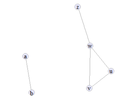
Consider this simple graph \(G\) with:
\(V(G) = \{w, v, u, z, a, b\}\)
\(E(G) = \{ \{v,w\}, \{v,u\}, \{u,w\}, \{w,z\}, \{a,b\}\)
A connected graph is a graph where there exists a path between any two vertices.
A disconnected graph has multiple components, meaning some vertices are not reachable from others.
is_connected(karate)A complete graph \(K_n\) is a simple graph where each pair of distinct vertices is connected by an edge. It has:
\[ |E(K_n)| = \frac{n(n-1)}{2} \]
edges.
g_complete <- make_full_graph(5)
plot(g_complete,
     vertex.color = "lavender")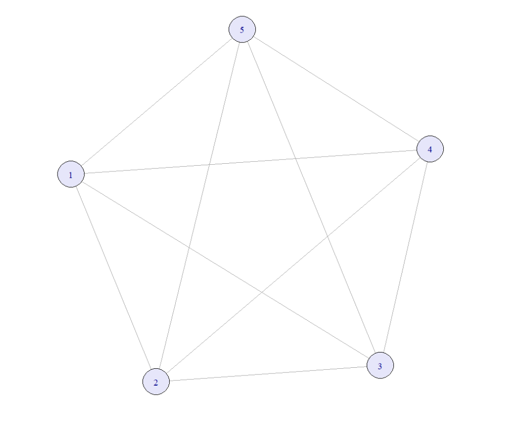
edge_density(make_empty_graph(20))
edge_density(make_full_graph(20))
\(1 =\) completely connected
\(0 =\) completely disconnected
Given an undirected Network \((V, E)\) a path of length \(l\) is a non-empty sequence of vertices \((v_1, v_2,..., v_{l+1})\), such that \(v_i \in V, \forall i = 1,...,l+1\) and \(v_i, v_{i+1} \in E \forall i = 1,...,l\) .
A path is simple if \(v_1 \neq v_j\) for all \(i<j\)
A path is closed if \(v_1 = v_{i+1}\)
A path is a cyle if it is closed and \(v_1 \neq v_j\) for all \(i<j\), except for the pair \((i,j) = (1, l+1)\)
A shortest path between two nodes is also called geodesic.
The (following) Zachary Karate Club data set is a very famous one, as it is publicly available and a good example for small-scale community structure analysis. Check Wikipedia for more information.
data(karate)


plot(karate)

sp <- shortest_paths(karate, 17)
sp$vpath[[24]]
path <- E(karate, path=sp$vpath[[24]])

# Set default colors and sizes
V(karate)$color <- "lavender"
E(karate)$color <- "lavender"
E(karate)$width <- 1

# Highlight path in pink
E(karate)[path]$color <- "pink"
E(karate)[path]$width <- 3

# Final plot
plot(karate)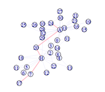
dist <- distances(karate)
dist
dist[1,] #expecting distances from node 1

E(karate)$weight # check the weightes in the network

dist <- distances(karate,
                  weights = rep(1,
                                ecount(karate)
                                )
                  ) #set weigths to 1
dist[1,]

distance_table(karate)
dist_tbl <- distance_table(karate)$res

barplot(dist_tbl,
        names.arg=1:length(dist_tbl)
        )
In undirected graphs the distance from node \(i\) to node \(j\) is the same as from \(j\) to \(i\). In directed graphs \(d(i,j)\) may not be equal \(d(j,i)\) and in some pairs even not reachable from one another.
\[ \bar{d} = \frac{1}{n(n-1)} \sum_{\substack{i,j = 1 \\ i \ne j}}^{n} d(i, j) \]
mean_distance(karate)[1] 5.754011
If the graph is disconnected, certain node pairs have no connecting path, leading to infinite distances. In such cases, the average is typically computed over all reachable pairs to avoid skewing the result
\[ \delta = max_{i,j}(d(i,j)) \]
max(dist)
diameter(karate,
         weights = rep(1,
                       ecount(karate)
                       )
         )
[1] 5
A subnetwork is a smaller part of a larger network. It includes a selection of nodes (vertices) and all the edges (connections) that exist between those selected nodes in the original network. Think of it like zooming in on a specific group within a bigger social network — for example, looking at just the group of friends connected to one person so a subnetwork is any network \(h=(W,F)\) where \(W \subseteq V\) and \(F \subseteq E\), containing all edges between nodes in \(W\).
A component is a subnetwork where every node is reachable from every other node, and which is not part of a larger connected subnetwork. In simpler terms, a component is a self-contained cluster — a group of nodes that are all connected to each other, but not to nodes outside the group.
So for example this graph has two components.
data(karate)


# Cutpoints
articulation_points(karate)

V(karate)$color <- "lavender"

V(karate)[articulation.points(karate)]$color <- "pink"
plot(karate)

components(karate)
karate_split <- delete_vertices(karate, c(1))
plot(karate_split)
components(karate_split)


E(karate)$color <- "lavender"

##  Set bridge edges to red:
num_comp <- length(decompose(karate))
for (i in 1:length(E(karate))) {
  karate_sub <- delete_edges(karate, i)
  if ( length(decompose(karate_sub) ) > num_comp ) E(karate)$color[i] <- "pink"
}

plot(karate)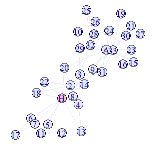
A network of size \(n\) is called k-connected if \(k < n\) and if it is connected even after removing any \(k − 1\) nodes. So you need to remove \(k\) nodes in order to disconnect the network.
Every connected network is at least 1-connected: You need to remove at least one node to disconnect the network.
If a network is \(k\)-connected, then the graph is also \((k - 1)\) connected: After removing \(k -1\) nodes, it is still connected.
k-components are the components a network is split into if you remove \(k\) nodes and split it into more than one component.
The greatest integer \(k\) such that the network is k-connected is known as the vertex-connectivity κ. If \(K = 0\), the network is disconected.
A cut set of a network is the set of nodes whose removal disconnects the graph. A minimum cut set is a smallest cut set.
Each minimum cut set contains \(K\) elements
A cutpoint exists if there is a minimum cut set of size \(1\).
There are many different forms of data collection for social network data. Options to collect data include Small Group questionnaires, large-scale Surveys, face-to-face observations, scraping of Websites, APIs or digital Archives. The choice of collection strategy has to be informed by the focus of research and available data sources. Almost always, when we are collecting network data, we are bounded by place and time where we have to make reasonable decisions in order to restrict our node set (Rawlings et al. 2023).
Collection strategies can broadly be structured in Local and Global collection strategies.
Local (Egocentric Networks)
Global (Sociocentric Networks)
Given the collection approach, there are different modes of collecting the data like the Nominalist Approach, which is based on observable links between actors
e.g.:
Co-authorship networks derived from Web of Science or Scopus.
Facebook-Connections
and the Realist Approach, which is based on self-reported relationships (e.g., surveys asking individuals to list friends).

Missing data in networks can bias results, particularly in global networks where completeness is crucial. Given the data collection choice and context, there can be different types of missing data:
Every form of data collection is prone to have some kinds of missing data, or inherent biases. Dealing with the possible consequences of the selected form of data collection and reporting possible biases and missings transparently is thus part of good scientific practice.

1. What is a relationship?
a) What counts as a relationship in network analysis?
b) Give three examples of relationships from your everyday life. For each:
c) What would you need to change to model these relationships differently? What effect could this have on your conclusions?
2. Networks beyond individuals
Define a network where events (not persons) are the nodes.
a) Give a concrete example
b) What would be the edges in this network?
c) How does this change the interpretation compared to person-based networks?
3. Research questions
Formulate two research questions that benefit from a social network analysis perspective.
4. Network boundaries
You study a friendship network in a master’s course.
a) How do you set the boundary of the network? Who is included, who isn’t? Why?
b) How do your decisions affect the structure of the network?
Now think about group work in this class. Discuss these three network representations:
c) Are these three different networks or one network with different types of edges?
d) How would you combine them? Does it make more sense to have directed or undirected edges? What information is lost in each case?
Try alone or in groups of two
1. Given this adjacency matrix:
\[ M = \begin{pmatrix} 0 & 1 & 0 & 1 & 0 & 1 \\ 1 & 0 & 0 & 1 & 0 & 1 \\ 0 & 0 & 0 & 1 & 0 & 1 \\ 0 & 0 & 0 & 0 & 0 & 1 \\ 0 & 1 & 0 & 1 & 0 & 1 \\ 1 & 0 & 0 & 1 & 0 & 0 \end{pmatrix} \] a) Create an igrap network object:
M <- matrix(c(
  0, 1, 0, 1, 0, 1,
  1, 0, 0, 1, 0, 1,
  0, 0, 0, 1, 0, 1,
  0, 0, 0, 0, 0, 1,
  0, 1, 0, 1, 0, 1,
  1, 0, 0, 1, 0, 0
  ),
  nrow = 6,
  byrow = TRUE
  )


g <- graph_from_adjacency_matrix(M,
                                 mode = "directed"
                                 )

plot(g)
b) How many edges and how many vertices does the network have?
vcount(g)
ecount(g)
c) Calculate the distances of node 3 to all other nodes. Interpret these values
dist <- distances(g, mode = "out")
dist
dist[3,]


#[1] 2 3 0 1 Inf 1 - the distance from node 3 to node 1 is 2, to node 2 its 3, there is a path of 0 to itself and no way to reach the vertex 5 (through out paths).
d) Find a command that gets you an edge list of the network.
eg <- as_edgelist(g)
eg
e) Use the indexication of the adjacency matrix to calculate the sum of outgoing and ingoing edges of node 6.
sum(M[,6]==1) # ingoing edges
sum(M[6,]==1) # outgoing edges
f) Is there a tie between vertex 2 and vertex 3?
are_adjacent(g, 2, 3)g) By changing the adjacency matrix, add an edge from vertex 5 to vertex 3.
M2 <- matrix(c(
  0, 1, 0, 1, 0, 1,
  1, 0, 0, 1, 0, 1,
  0, 0, 0, 1, 0, 1,
  0, 0, 0, 0, 0, 1,
  0, 1, 1, 1, 0, 1,
  1, 0, 0, 1, 0, 0
), nrow = 6, byrow = TRUE)

g2 <- graph_from_adjacency_matrix(M2)
plot(g2)
2. Given the following dataset:
df <- data.frame(id = c(1:10),
                 friend1 = c(9, 8, 10,  3,  1,  4,  2,  6,  7,  5), # first friend nomination
                 friend2 = c(5, 7, 2, 2, 3,  7,  3, 10,  1, 8),  # second friend nomination
                 friend3 = c(NA, NA, 4, 6, 10, 8, 5, NA, NA, 3), # third friend nomination
                 age = c(15, 15, 15, 16, 14, 14, 14, 15, 16, 14), # age in years
                 gender = c(2, 0, 1, 0, 1, 1, 2, 0, 0, 1)) # gender: 0= male, 1= female, 2= divers
a) Create a network object*
edges1 <- data.frame(from = df$id,
                     to = df$friend1)

edges2 <- data.frame(from = df$id,
                     to = df$friend2)

edges3 <- data.frame(from  = df$id,
                     to = df$friend3)

# Combine all edges into one data frame
edges <- rbind(edges1, edges2, edges3)

# Remove rows with NA (where there was no third friend)
edges <- na.omit(edges)

# Create graph from edge list and vertex attributes
g <- graph_from_data_frame(d = edges, directed = TRUE, vertices = df)

plot(g)
b) Add the vertex attributes gender and age.
# Set vertex attributes
V(g)$name <- df$id
V(g)$age <- df$age
V(g)$gender <- df$gender

scaled_age <- scales::rescale(V(g)$age, to = c(5, 20))

# Optional: plot the graph with attributes
plot(g,
     vertex.label = V(g)$name, # use "name" for labels
     vertex.size = scaled_age,
     vertex.color = ifelse(V(g)$gender == 0, "lightblue",
                    ifelse(V(g)$gender == 1, "pink", "purple")),
     edge.arrow.size = 0.5,
     main = "Friendship Network with Age and Gender")
d) Think about data storage and representation. When is the dataframe more useful, when is the graph object more useful? When would you use an adjacency matrix instead?
Social networks
A social network consists of a set of actors that are connected by relationships in a pairwise manner (Wasserman and Faust 2009). Actors can represent individuals, groups, organizations, companies, or even entire countries. The nature of these relationships varies and can be defined in different ways, such as:
Networks are commonly visualized in plots by nodes (usually circles), representing the actors and edges (lines or arrows) , representing the relationships.
Code