Weekly preparation

Code

library(needs)

needs(tidyverse,
      dplyr,
      stopwords,
      SnowballC,
      jsonlite,
      tidytext,
      udpipe,
      ggwordcloud,
      stopwords
      )

Text as Data

Different text as a form of data has been around since the beginning of the social sciences. Qualitative data, such as interviews, field notes, and historical documents, have always been a rich source of information for social scientists. However, with the advent of digital technology and the internet, the amount of text data available has exploded, leading to new opportunities and challenges for social scientists.

But, with large-scale data, we need to be able to analyze it in a systematic and efficient way. This is where computational methods for text analysis come in. By using techniques from natural language processing (NLP) and machine learning, we can extract insights from large collections of text data that would be impossible to analyze manually.

We are, in some way, trying to quantify the qualitative.

Key concepts:

For the computational analysis of text, machines need to be able to work with text data in a structured way. This involves breaking down text into smaller units and representing it in a format that can be analyzed quantitatively.

Document: A single text unit, such as an article, a speech, or a tweet.
Corpus: A collection of documents.
Token: The basic unit (word, punctuation, number)

On a side note: Different text sources and elements need different pre-processing and methods. For example: while some tasks work great for speeches or letters, they will not work for tweets or forum posts, as they differ significantly in style, length, and content. So it is important to consider the specific characteristics of the text data you are working with when choosing methods for analysis. Text data analysis (as well as any data analysis really) has to always be guided by the research question and the specific context of the data.

Text Manipulation with `stringr`

Let’s start with a simple example of a character string and a vector of character strings.

Code

string_vector <- c(
  "We all love data science and of course we love sociology!",
  "Data science is great, but I also love sociology.",
  "Sociology and data science are both fascinating fields.",
  "I love this course. It is fantastic",
  "This assignment is terrible and frustrating."
)

documents <- tibble(
  doc_id = 1:length(string_vector),
  text = string_vector
)

Using the r package stringr we can manipulate these character strings in various ways. We will cover some of the most common functions for text manipulation (or any working with character strings.i.e sequences of characters.

The stringr package is included in the tidyverse, which I highly recommend getting used to in general for data manipulation and analysis in R.

All stringr-commands begin with str_ and are very intuitive to use.

All stringr-functions are vectorized, which means that they can be applied to a vector of character strings and will return a vector of the same length with the results. This makes it easy to work with large datasets of text data. The commands are case sensitive though!

Detect matches

str_detect(string,*pattern*): Detects if a pattern exists in a string. Returns TRUE or FALSE.
str_which(string,*pattern*): Returns the indices of the strings that contain the pattern.
str_count(string,*pattern*): Counts the number of times a pattern appears in a string.
str_locate(string,*pattern*): Returns the starting and ending positions of the first match of the pattern in the string. Also str_locate_all for all matches.

Code

str_detect(string_vector, "data")

str_which(string_vector, "data")

str_which(string_vector, "Data")

str_count(string_vector, "love")

str_locate(string_vector, "data")

str_locate_all(string_vector, "data")

We can also do these manipulations on a dataframe or tibble by using mutate() and applying the stringr functions to the relevant columns.

Code

documents |>
  mutate(
    start = str_locate(text, "data")[,1],
    end   = str_locate(text, "data")[,2]
  )

Subset strings

str_sub(string, start=1L, end=-1L): Extracts a substring from a string based on the specified start and end positions.
str_subset(string,*pattern*): Returns the strings that contain the pattern.
str_extract(string,*pattern*): Extracts the first match of a pattern from a string. Also str_extract_all for all matches.
str_match(string,*pattern*): Returns the first pattern match found in each string, as a matrice with a column for each () group in pattern. Also str_match_all for all matches.

Code

str_sub(string_vector, start=1, end=10)

str_subset(string_vector, "sociology")

str_extract(string_vector, "data")

str_extract_all(string_vector, "data")

str_match(string_vector, "data (\\w+)")

str_match_all(string_vector, "data (\\w+)")

Manage lengths

str_length(string): Returns the number of characters in a string.
str_pad(string, width, side = c("left", "right", "both"), pad = " "): Pads a string to a specified width with a specified character.
str_trunc(string, width, side = c("left", "right", "center"), ellipsis = "..."): Truncates a string to a specified width, adding an ellipsis if the string is too long.
str_trim(string, side = c("both", "left", "right")): trims whitespace from the start and/or end of a string.

Code

str_length(string_vector)

str_pad(string_vector, width = 35, side = "right", pad = ".")

str_trunc(string_vector, width = 41, side = "right", ellipsis = "...")

str_trim("   This string has extra spaces.   ")

Mutate strings

str_sub() <- value: Replace substrings by identifying the substrings with str_sub() and then assigning new values to them.
str_replace(string, pattern, replacement): Replaces the first match of a pattern in a string with a replacement. Also str_replace_all for all matches.
str_to_lower(string): Converts a string to lowercase.
str_to_upper(string): Converts a string to uppercase.
str_to_title(string): Converts a string to title case (first letter of each word capitalized).

Code

str_sub(string_vector[1], start=1, end=2) <- "We all love data science and of course we love sociology!"

str_sub(string_vector[1], start=3, end=58) <- " "

str_replace(string_vector, "data", "DATA")

str_replace_all(string_vector, "data", "DATA")

str_to_lower(string_vector)

str_to_upper(string_vector)

str_to_title(string_vector)

Join and Split strings

str_c(..., sep = " ", collapse = NULL): Concatenates strings together with a specified separator. If collapse is not NULL, it will concatenate the results into a single string.
str_dup(string, times): Duplicates a string a specified number of times.
str_split_fixed(string, pattern, n): Splits a string into a matrix of substrings (splitting at occurences of a pattern match). Also str_split()to return a list of substrings.

Regexes

Regular expressions (regex) are patterns used to search, match, and manipulate text. Instead of searching for fixed strings like "data", regex allows you to describe patterns such as:

any digit
a word starting with a capital letter
three letters followed by two numbers
a word at the end of a sentence

Regex is extremely powerful for text analysis, data cleaning, or general computational social science applications.

So basically a regular expression is a pattern description language. When we write str_detect(string_vector, "data"), we are using a regular expression to search for the exact string “data”.

Core Regex Building Blocks

Literals

Literal Characters are the most basic building blocks of regular expressions. They match themselves exactly. For example, the regex data will match the string “data” in any text.

Character Classes

/TODO - Harmonize list

Character classes define what kind of character you want.

Pattern	Meaning
.	any character except newline
\d	digit (0-9)
\D	non-digit
\w	word character (letters, digits, underscore)
\W	non-word character
\s	whitespace character (space, tab, newline)
\S	non-whitespace character

Example: str_detect(string_vector, "\\d") will return TRUE for any string that contains a digit.

There are several abbreviations in stringr for easier text manipulation:

[[:punct:]: all punctuation characters from a string.
[[:digit:]]: all digits from a string.
[[:space:]]: whitespace characters with a single space.
[[:alpha:]]: all alphabetic characters from a string.
[[:alnum:]]): all alphanumeric characters from a string.
[[:graph:]]): all visible characters (letters, digits, punctuation) from a string.
[[:print:]]: all printable characters (letters, digits, punctuation, space) from a string.

Custom Character Set

You can define your own character groups:

Pattern	Meaning
[abc]	matches any one of the characters a, b, or c
[a-z]	matches any lowercase letter
[A-Z]	matches any uppercase letter
[0-9]	matches any digit
[^abc]	matches any character that is not a, b, or c

Quantifiers

Quantifiers specify how many times a character or group should be matched.

Pattern	Meaning
*	0 or more times
+	1 or more times
?	0 or 1 time
{n}	exactly n times
{n,}	n or more times
{n,m}	between n and m times

Example: "\\d+" will match any sequence of one or more digits.

5 will match
123 will match
abc will not match

Anchors

Anchors define where something occurs.

Pattern	Meaning
^	start of the string
$	end of the string
\b	word boundary

Example: "^Data" matches strings that start with “Data” and "science$" matches strings that end with “science”.

Grouping

Parantheses () group parts of a pattern together. This is useful for applying quantifiers to a group of characters or for extracting specific parts of a match.

Example: (abc)+ will match one or more occurrences of the sequence “abc”. So it will match “abc”, “abcabc”, “abcabcabc”, etc.

Alternation

The pipe | allows you to match one pattern or another. For example, cat|dog will match either “cat” or “dog”.

Escaping special characters

Some characters have special meanings:

. * + ? ^ $ ( ) [ ] { } | \

If you want to match them literally, you must escape them:

\\. \\* \\+ \\? \\^ \\$ \$ \$ \\[ \\] \\{ \\} \\| \\\\

Special escape characters in R

In R you write regular expressions as strings. (“” or ’’). Some characters cannot be represented directly in an R string. These bust be represented as special characters

Character	Description
`\\`	`\`
`\"`	`"`
`\n`	Newline

You can run ?"'" to see a complete list

Greedyness

Regex is greedy by default, which means it will match as much of the string as possible. For example, the regex a.*b will match the longest string that starts with “a” and ends with “b”. If you want to make it non-greedy (match as little as possible), you can use ? after the quantifier: a.*?b.

Example: In the string “aXbYb”, a.*b will match “aXbYb” (greedy), while a.*?b will match “aXb” (lazy).

In-class exercise

Download data as presidential speeches from Miller Center of Public Affairs as bulk download. Click link, scroll all the way down, hit *Download Millercenter.org Data* and save the file. Unpack it and find the folder speeches with all the JSON files in it. We will use this data for our exercises for these two sessions.

Collecting data

Using bulk download is a common way to collect data when you have a large number of files to download. It allows you to download all the files at once, rather than having to download each file individually. This can save you a lot of time and effort, especially if you have a large number of files to download. However it is not always available, and sometimes you have to use other methods to collect data, such as web scraping or using APIs. We will briefly discuss different ways to access data in the last session of the seminar.

Once you downloaded the data run the following code to create a dataframe with all the speeches. The code reads all the JSON files in the speeches folder, identifies all unique keys across the JSON files, and creates a dataframe where each row corresponds to a speech and each column corresponds to a key from the JSON files. If a key is missing in a particular JSON file, it will be filled with NA in the dataframe.

Code

# Folder containing your JSON files
json_folder <- "C:\\Users\\ls68bino\\Documents\\GitHub\\leostnbrk.github.io\\data\\presidential speeches\\speeches"

#json_folder <- "path/to/your/speeches/folder" 

# List all JSON files in the folder
json_files <- list.files(json_folder,
                         pattern = "\\.json$",
                         full.names = TRUE)

# Function to read a JSON and convert it to a named list
read_json_as_list <- function(file) {
  fromJSON(file,
           simplifyVector = FALSE
           ) # keep as list
}

# Read all JSONs
json_data <- lapply(json_files,
                    read_json_as_list)

# Identify all unique keys across all JSONs
all_keys <- unique(unlist(lapply(json_data,
                                 names
                                 )
                          )
                   )

# Convert each JSON list to a dataframe, ensuring all columns exist
json_dfs <- lapply(json_data,
                   function(x) {
  # Add missing keys as NA
  missing_keys <- setdiff(all_keys,
                          names(x)
                          )
  if (length(missing_keys) > 0) {
    x[missing_keys] <- NA
  }
  as.data.frame(x,
                stringsAsFactors = FALSE
                )
})

# Combine all into one dataframe
final_df <- bind_rows(json_dfs)

final_df_backup <- final_df # backup in case we mess up the data

Use regexes to clean the title of the speeches, so that they only contain the name: March 25, 2021: First Press Conference should be only “First Press Conference”.
Clean up the dates, so they remain in this format: YYYY-MM-DD.
Change speeches to lowercase.
If needed, remove any html artefacts from the text of the speeches.

Code

final_df <- final_df |>
  mutate(title = str_replace(title, "^.*?:\\s*", "")) |>
  mutate(date = str_sub(date, 1, 10)) |>
  mutate(transcript = str_to_lower(transcript))
  



html_pattern <- "<.*?>|&nbsp;"
str_detect(final_df$transcript, html_pattern) 

final_df <- final_df |>
  mutate(transcript = str_replace_all(transcript, html_pattern, "")) |>
  mutate(transcript = str_trim(transcript))

Further text manipulation

Tokenization

Tokenization is the process of splitting text into smaller units called tokens. Tokens are usually words, but they can also be sentences, characters, or n-grams. Tokenization is typically the first stel in any NLP pipeline, as it allows us to work with individual words or other units of text. In R, tokenization works very well with the tidytext package, which provides a set of functions for tokenizing text data.

Code

tokens <- documents |>
  unnest_tokens(word, text)

tokens

Stemming

Stemming is the process of reducing words to their base or root form. It is a common technique in natural language processing (NLP) to simplify text data and reduce the number of unique words in a corpus. For example, the words “running”, “runner”, and “ran” can all be reduced to the stem “run”. This can help improve the performance of NLP models by reducing the dimensionality of the data and allowing the model to focus on the core meaning of the words rather than their specific forms. This is of course only helpful, it we aren’t interested in the specific forms of the words (e.g. sociology, sociologists, sociological) but rather in the general concept (sociology). Stemming can be done using various algorithms, such as the Porter Stemmer (you can call this by using language = "porter) or the Snowball Stemmer, which apply a set of rules to determine how to reduce words to their stems.

In R we can use the SnowballC package to perform stemming. The wordStem() function takes a vector of words and returns their stems.

Most stemming algorithms are designed for English, but there are also algorithms for other languages. The SnowballC package supports several languages, including English, Spanish, French, German, and more. You can specify the language using the language argument in the wordStem() function. For example,wordStem(words, language = "german") will stem German words. BUT: As you can see below, the german stemming is far from perfect, but it does reduce the words to their base forms to some extent.

Code

words <- c("running", "run", "runner", "ran", "runners", "runs")
print(wordStem(words))


words_2 <- c("sociology", "sociologist", "sociological")
print(wordStem(words_2))



words_german <- c("Häuser", "Haus", "häuslich", "hausen", "Häuserreihe", "Häuschen")
print(wordStem(words_german, language = "german"))

Lemmatization

Lemmatization reduces words to their dictionary base form (lemma)*. Unlike stemming, it uses linguistic knowledge and considers the grammatical role of a word.

Lemmatization is usually more accurate than stemming because it produces real words and handles irregular forms properly. However, it requires more computational resources and language models.

In R, lemmatization can be performed using the udpipe-package.

Lemmatization depends on language-specific models. The udpipe package supports many languages, but you must download and load the appropriate model first (e.g., English, German, French, etc.).

Code

# downliad once (if needed)
lemma_eng <- udpipe_download_model(language = "english")
ud_model <- udpipe_load_model(lemma_eng$file_model)

lemma_deu <- udpipe_download_model(language = "german")
ud_model_deu <- udpipe_load_model(lemma_deu$file_model)



text <- "running runner ran runners runs"
lemma_result <- udpipe_annotate(ud_model, x = text)
lemma_result_df <- as.data.frame(lemma_result)
print(lemma_result_df$lemma)

text_deu <- "Häuser Haus häuslich hausen Häuserreihe Häuschen"
lemma_result_deu <- udpipe_annotate(ud_model_deu, x = text_deu)
lemma_result_deu_df <- as.data.frame(lemma_result_deu)
print(lemma_result_deu_df$lemma)

text_2 <- "sociology sociologist sociological social sociologists"
lemma_result_2 <- udpipe_annotate(ud_model, x = text_2)
lemma_result_2_df <- as.data.frame(lemma_result_2)
print(lemma_result_2_df$lemma)

Stopwords

Stopwords are very common words that usually carry little semantic meaning (e.g., “the”, “and”, “is”). Removing them can reduce noise and improve many NLP tasks. In R, stopword lists are available through the stopwords-package.

Code

# English stopwords
stopwords("en")[1:30]

# German stopwords
stopwords("de")[1:30]

We can either use these full lists or create own lists of stopwords based on our specific needs. For example, if we are analyzing presidential speeches, we might want to add words like “president”, “speech”, “america”, etc. to our stopword list, as they are likely to be very common and not carry much meaning in the context of our analysis. But we might be interested in keeping words like “they” or “we”, as they can be important for understanding the content of the speeches. So it really depends on the specific context and research question of our analysis.

We can remove stopwords after tokenization by using an anti_join with the stopword list. This will keep only the tokens that are not in the stopword list.

Code

tokens_clean <- tokens |>
  filter(!word %in% stopwords("en"))

tokens_clean

Bag of Words

Bag of words: A bag of words is a (vector)-representation of text that describes the occurrence of words within a document. It is a simplified model that disregards grammar and word order but keeps track of the frequency of each word.

We think of a document $d_j$ as a bag of words. Let $f_j(w_i)$ be the frequency of word $w_i$ in document $d_j$. Then we can represent document $d_j$ as a vector of word frequencies.

\[ d_j = \{f(w_1), f(w_2), ..., f(w_n)\} \]

Example:

$d_i$ = “We all love data science and of course we love sociology!”

Word	Frequency
all	1
and	1
course	1
data	1
love	2
of	1
science	1
sociology	1
we	2

Assumptions of the bag of words model:

Each word contributes equally to the text
The order of words does not matter

Document x Term/Feature Matrix

A Document-Feature Matrix (DFM) is an important format for analyzing text data.

It is (no shit, Sherlock) in the form of a matrix, in which the texts (documents) are in the rows and the words, characters, etc. (features) are in the columns. The cells count how often a feature occurs in the respective text.

Code

tokens <- documents |>
  unnest_tokens(word, text)


tokens <- tokens |>
  anti_join(stop_words, by = "word")

dfm <- tokens |>
  count(doc_id, word) |>
  pivot_wider(
    names_from = word,
    values_from = n,
    values_fill = 0
  )

Visualisation

Feature Frequencies

Code

tokens |>
  count(word, sort = TRUE) |>
  slice_max(n, n = 10) |>
  ggplot(aes(reorder(word, n), n)) +
  geom_col(fill = "lightblue") +
  coord_flip() +
  labs(x = NULL, y = "Frequency")

Heatmaps

Code

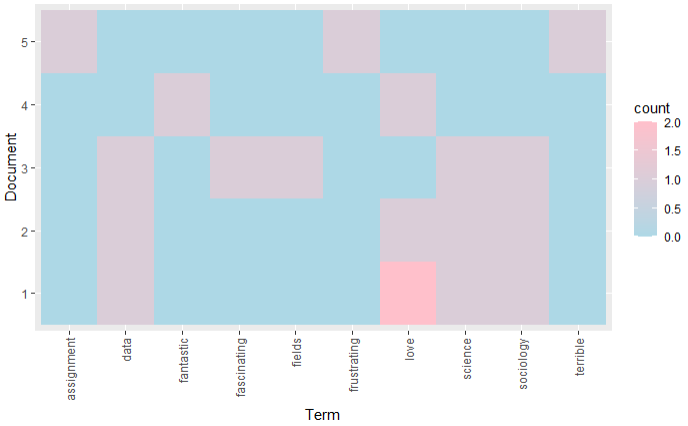
dfm_long <- dfm |>
  pivot_longer(-doc_id, names_to = "word", values_to = "count")

ggplot(dfm_long, aes(x = word, y = factor(doc_id), fill = count)) +
  geom_tile() +
  scale_fill_gradient(low = "lightblue", high = "pink") +
  labs(y = "Document", x = "Term") +
  theme(
    axis.text.x = element_text(angle = 90, vjust = 0.5, hjust = 1),
  )

Wordclouds

Code

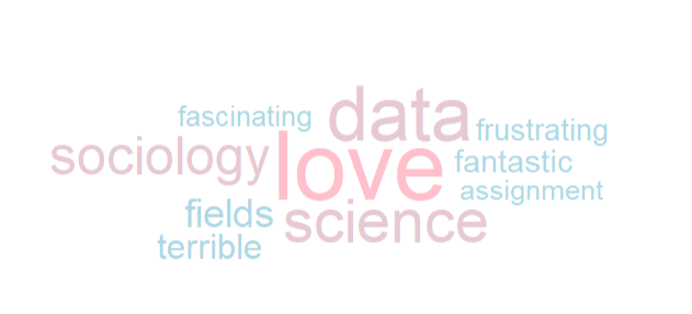
tokens |>
  count(word, sort = TRUE) |>
  ggplot(aes(label = word, size = n, color = n)) +
  geom_text_wordcloud_area() +
  scale_size_area(max_size = 40) +
  scale_color_gradient(low = "lightblue", high = "pink") +
  theme_minimal() +
  theme(
    legend.position = "none",
    plot.background = element_rect(fill = "white", color = NA)
  )

Week 07 - Text analysis I

Weekly preparation

Text as Data

Key concepts:

Text Manipulation with `stringr`

Detect matches

Subset strings

Manage lengths

Mutate strings

Join and Split strings

Regexes

Core Regex Building Blocks

Literals

Character Classes

Custom Character Set

Quantifiers

Anchors

Grouping

Alternation

Escaping special characters

Special escape characters in R

Greedyness

In-class exercise

Collecting data

Further text manipulation

Tokenization

Stemming

Lemmatization

Stopwords

Bag of Words

Document x Term/Feature Matrix

Visualisation

Feature Frequencies

Heatmaps

Wordclouds

Copyright

Weekly preparation

Text as Data

Key concepts:

Text Manipulation with stringr

Detect matches

Subset strings

Manage lengths

Mutate strings

Join and Split strings

Regexes

Core Regex Building Blocks

Literals

Character Classes

Custom Character Set

Quantifiers

Anchors

Grouping

Alternation

Escaping special characters

Special escape characters in R

Greedyness

In-class exercise

Collecting data

Further text manipulation

Tokenization

Stemming

Lemmatization

Stopwords

Bag of Words

Document x Term/Feature Matrix

Visualisation

Feature Frequencies

Heatmaps

Wordclouds

Copyright

Text Manipulation with `stringr`