Great, what can we do with this cleaned up data now?
Code
string_vector <-c("We all love data science and of course we love sociology!","Data science is great, but I also love sociology.","Sociology and data science are both fascinating fields.","I love this course. It is fantastic","This assignment is terrible and frustrating.")documents <-tibble(doc_id =1:length(string_vector),text = string_vector)
Tf-idf
The Tf-idf (term frequency-inverse document frequency) is a numerical statistic that reflects how important a word is to a document in a collection or corpus. It is often used as a weighting factor in information retrieval and text mining.
The main idea is: - Words appear often in one document are important for the document - Words that appear in many documents are less important overall.
\(f_{t,d}\) be the number of times term \(t\) appears in document \(d\)
The simplest definition is raw term frequency:
\[
\text{tf}(t, d) = f_{t,d}
\]
Often we use a normalized version to account for document length: \[
\text{tf}(t, d) = \frac{f_{t,d}}{\sum_{t' \in d} f_{t',d}}
\]
where the deniminator is the total number of terms in document \(d\). This prevents longer documents from automatically having higher term frequencies.
Inverse Document Frequency (IDF)
Let: - \(N\) be the total number of documents in the corpus \(D\) - \(df_t\) be the number of documents in which term \(t\) appears
The standard definition is: \[
\text{idf}(t, D) = \log\left(\frac{N}{df_t}\right)
\]
With the interpretation: - If \(df_t = N\): \[
\text{idf}(t, D) = \log(1) = 0
\] with no discriminating power.
Topic modeling is a technique used to identify and extract the most important themes (topics) from a collection of documents (corpus). It is based on the idea that documents are mixtures of topics, and that topics are distributions over words.
Little prior knowledge about the content is needed
Questions we can ask ourselves with the help of topic models:
What are the main themes in a collection of documents?
How do these themes evolve over time?
How do different documents relate to each other based on their thematic content?
How do texts differ in their content?
Assumptions of Topic Modeling
Topic modeling also builds on the bag of words idea from last week, which means that it does not take into account the order of words in a document and assumes, that all words contribute equally to the text
Each text consists of a mixture of different topics (with different proportions)
Texts that discuss similar topics use similar words
The Algorithm
Two Steps: - Finding out which words occur together - Checking how these words are distributed among the texts - Unsupervised machine learning, since we do not have any labels for the topics in the documents
We have to tell the algorithm how many topics we want to find, and it will then assign each word to a topic and each document to a mixture of topics.
-Iterative process designed to maximize two goals simulateously: words that occur together frequently are more likely to belong to the same topic.Words that occur in the same document are more likely to belong to the same topic.
TODO
Interpretation and Limitations
Sentiment Analyis
Sentiment analysis is a method used in natural language processing (NLP) to measure the emotional tone of a text. The goal is typically to classify text as positive, negative, or sometimes neutral. More fine-grained approaches can detect specific emotions such as joy, anger, fear, or trust.
For example: - Good, excellent, happy –> positive sentiment - Bad, terrible, sad –> negative sentiment
With this we can (try to) answer questions like:
What is the public opininion on a certain topic?
How do people feel about a certain product or service?
How do people feel about a certain event? (You get the point)
Dictionary based approaches
In computational text analysis, sentiment analysis is often lexicon-based. This means that words are compared to predefined dictionaries that assign sentiment scores or emotional categories.
For example, some sentiment dictionaries are integrated in tidytext.
"bing"- positive/negative classification
afinn - numeric sentiment score ranging from -5 (negative) to +5 (positive) - only in package textdata
"nrc" - categorizes words into 8 emotions (anger, anticipation, disgust, fear, joy, sadness, surprise, trust) and 2 sentiments (positive, negative)
Code
library(textdata)text_df <-tibble(text = string_vector)tokens <- text_df |>unnest_tokens(word, text)sentiment_bing <-get_sentiments("bing")sentiment_afinn <-get_sentiments("afinn")sentiment_nrc <-get_sentiments("nrc")tokens_bing <- tokens |>inner_join(sentiment_bing, by ="word")tokens_afinn <- tokens |>inner_join(sentiment_afinn, by ="word")tokens_nrc <- tokens |>inner_join(sentiment_nrc, by ="word")
One of the biggest german sentiment lexica was developed at Leipzig University and is called SentiWS (Remus, Quasthoff, and Heyer 2010). It contains around 3000 positive and negative words, including their inflected forms. The lexicon is freely available for research purposes and can be downloaded here
Which president has the highest sentiment? Chose your method.
Limitations
Because, we connect tokens to a dictionary, we can only analyze the sentiment of words that are included in the dictionary. This means that if a word is not in the dictionary, it will not be analyzed for sentiment. This can lead to incomplete or inaccurate sentiment analysis, especially if the text contains many words that are not in the dictionary. There are data sources that are more likely to be included in these dictionaries, such as product reviews or political speeches, and others that are less likely to be included, such as social media posts, or other fast evolving speech areas.
Word embeddings
Bag of Words
Word2Vec
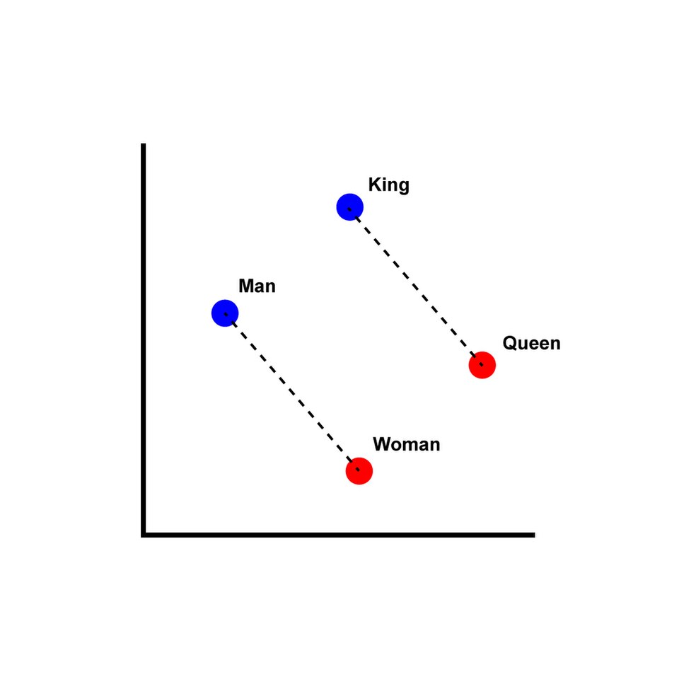
Word2Vec (Mikolov et al. 2013) is a neural embedding model that represents words as dense numeric vectors. Unlike the approaches above, that count word frequencies, Word2Vec learns word meaning from context.
Core idea: Words that appear in similar contexts will have similar vector representations.
Word2Vec-Example
Word2Vec uses a shallow neural network to learn these vector representations. The model is trained on a large corpus of text, and it learns to predict a word based on its surrounding words (context). The resulting word vectors capture semantic relationships between words, such that words with similar meanings will have similar vector representations.
In R, we can use the word2vec package.
TODO:
Code
# Tokenize sentences into word liststokens <- text_df |>unnest_tokens(word, text) |>group_by(doc_id) |>summarise(text =paste(word, collapse =" "))# Train modelmodel <-word2vec(x = tokens,type ="skip-gram",dim =50,window =5,iter =20)# Inspect embeddingsembeddings <-as.matrix(model)head(embeddings)# Get word vectorsembeddings <-as.matrix(model)
Word2Vecs nees much larger corpora to work well. The example above is just for illustrative purposes. In practice, you would need to train the model on a much larger corpus of text to get meaningful word embeddings.
There is no real R-implementation of more recent embedding models, such as BERT or GPT, but we can use the sentence-transformers library in Python to get sentence embeddings.
There are various ways of measuring the similarity of text embeddings. One common method is to use cosine similarity, which measures the cosine of the angle between two vectors in a multi-dimensional space. The cosine similarity ranges from -1 to 1, where 1 means that the vectors are identical, 0 means that they are orthogonal (i.e., they have no similarity), and -1 means that they are diametrically opposed.
Code
from sentence_transformers import SentenceTransformermodel = SentenceTransformer("all-MiniLM-L6-v2") # Modellauswahls1 ="Computational Social Science uses machine learning to analyze social data."s2 ="Machine learning methods are central to computational social science research."s3 ="I enjoy cooking Italian pasta with fresh tomatoes and basil."s4 ="The Bundesliga season starts next weekend."s5 ="I enjoy cooking Italian pasta with fresh tomatoes and basil."emb1 = model.encode(s1)emb2 = model.encode(s2)emb3 = model.encode(s3)emb4 = model.encode(s4)emb5 = model.encode(s5)model.similarity(emb1, emb2)model.similarity(emb1, emb3)model.similarity(emb1, emb4)model.similarity(emb3, emb5)
library(plotly)df <- reticulate::py$dfplot_ly(df, x =~x, y =~y, z =~z, text =~word, type ="scatter3d", mode ="markers+text") %>%layout(scene =list(xaxis =list(title ="PC1"),yaxis =list(title ="PC2"),zaxis =list(title ="PC3") ))
]
Aufgabe:
Es gibt verschiedene
References
Mikolov, Tomas, Kai Chen, Greg Corrado, and Jeffrey Dean. 2013. “Efficient Estimation of Word Representations in Vector Space.” arXiv. https://doi.org/10.48550/arXiv.1301.3781.
Remus, Robert, Uwe Quasthoff, and Gerhard Heyer. 2010. “SentiWS - A Publicly Available German-language Resource for Sentiment Analysis.” In Proceedings of the International Conference on Language Resources and Evaluation, LREC 2010, 17-23 May 2010, Valletta, Malta.
 ]
]